Rcmdr.kr: An R Commander User in Korea

통계 > 적합성 모델 > 서열(Ordinal) 회귀 모델...
Statistics > Fit models > Ordinal regression model...

MASS 패키지에 있는 housing 데이터셋을 활용해보자. 먼저 housing 데이터셋을 활성화 시킨다. https://rcmdr.tistory.com/215

Sat는 거주자의 현 거주환경에 대한 만족도에 관한 변수로서, High > Medium > Low 라는 서열화된 요인을 갖고 있다. Sat를 반응변수로, 나머지를 설명변수의 후보군으로 모델을 구성하는 것이다. Freq 변수는 Sat, Infl, Type, Cont 등으로 구별되는 집단 구성원의 숫자를 뜻한다. 아래와 같이 모형을 만든다.

OrdRegModel.1 <- polr(Sat ~ Infl + Type + Cont , weights = Freq, method="logistic", 
  data=housing, Hess=TRUE)
summary(OrdRegModel.1)

OrdRegModel.1 이라는 모형이 만들어졌다면, '모델 > 가설 검정 > 분산분석표...' 메뉴 기능을 이용할 수 있다.

MASS::housing()

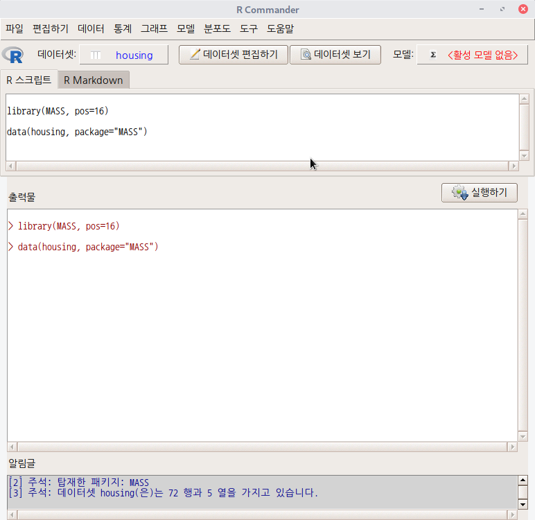
library(MASS, pos=16)
data(housing, package="MASS")

'도구 > 패키지 적재하기...' 메뉴 기능을 선택하고, MASS 패키지를 찾아서 선택한다.

그리고나서, '데이터 > 패키지에 있는 데이터 > 첨부된 패키지에서 데이터셋 읽기...' 메뉴 기능을 선택하면 하위 선택 창으로 이동한다. 아래와 같이 MASS 패키지를 선택하고, housing 데이터셋을 찾아 선택한다.

housing 데이터셋이 활성화된다. R Commander 상단의 메뉴에서 < 활성 데이터셋 없음> 이 'housing'로 바뀐다.

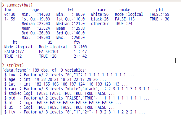
summary(housing)
str(housing)

'통계 > 요약 > 활성 데이터셋' 메뉴 기능을 선택하여 housing 데이터셋의 요약 정보를 살펴보자. 아울러 입력창에 str(housing)을 입력하고 <실행하기> 버튼을 누르자.

데이터셋의 내부는 다음과 같다:

Frequency Table from a Copenhagen Housing Conditions Survey

Description

The housing data frame has 72 rows and 5 variables.

Usage

housing

Format

Sat

Satisfaction of householders with their present housing circumstances, (High, Medium or Low, ordered factor).

Infl

Perceived degree of influence householders have on the management of the property (High, Medium, Low).

Type

Type of rental accommodation, (Tower, Atrium, Apartment, Terrace).

Cont

Contact residents are afforded with other residents, (Low, High).

Freq

Frequencies: the numbers of residents in each class.

Source

Madsen, M. (1976) Statistical analysis of multiple contingency tables. Two examples. Scand. J. Statist. 3, 97–106.

Cox, D. R. and Snell, E. J. (1984) Applied Statistics, Principles and Examples. Chapman & Hall.

References

Venables, W. N. and Ripley, B. D. (2002) Modern Applied Statistics with S. Fourth edition. Springer.

Examples

options(contrasts = c("contr.treatment", "contr.poly"))

# Surrogate Poisson models
house.glm0 <- glm(Freq ~ Infl*Type*Cont + Sat, family = poisson,
                  data = housing)
## IGNORE_RDIFF_BEGIN
summary(house.glm0, cor = FALSE)
## IGNORE_RDIFF_END

addterm(house.glm0, ~. + Sat:(Infl+Type+Cont), test = "Chisq")

house.glm1 <- update(house.glm0, . ~ . + Sat*(Infl+Type+Cont))
summary(house.glm1, cor = FALSE)

1 - pchisq(deviance(house.glm1), house.glm1$df.residual)

dropterm(house.glm1, test = "Chisq")

addterm(house.glm1, ~. + Sat:(Infl+Type+Cont)^2, test  =  "Chisq")

hnames <- lapply(housing[, -5], levels) # omit Freq
newData <- expand.grid(hnames)
newData$Sat <- ordered(newData$Sat)
house.pm <- predict(house.glm1, newData,
                    type = "response")  # poisson means
house.pm <- matrix(house.pm, ncol = 3, byrow = TRUE,
                   dimnames = list(NULL, hnames[[1]]))
house.pr <- house.pm/drop(house.pm %*% rep(1, 3))
cbind(expand.grid(hnames[-1]), round(house.pr, 2))

# Iterative proportional scaling
loglm(Freq ~ Infl*Type*Cont + Sat*(Infl+Type+Cont), data = housing)


# multinomial model
library(nnet)
(house.mult<- multinom(Sat ~ Infl + Type + Cont, weights = Freq,
                       data = housing))
house.mult2 <- multinom(Sat ~ Infl*Type*Cont, weights = Freq,
                        data = housing)
anova(house.mult, house.mult2)

house.pm <- predict(house.mult, expand.grid(hnames[-1]), type = "probs")
cbind(expand.grid(hnames[-1]), round(house.pm, 2))

# proportional odds model
house.cpr <- apply(house.pr, 1, cumsum)
logit <- function(x) log(x/(1-x))
house.ld <- logit(house.cpr[2, ]) - logit(house.cpr[1, ])
(ratio <- sort(drop(house.ld)))
mean(ratio)

(house.plr <- polr(Sat ~ Infl + Type + Cont,
                   data = housing, weights = Freq))

house.pr1 <- predict(house.plr, expand.grid(hnames[-1]), type = "probs")
cbind(expand.grid(hnames[-1]), round(house.pr1, 2))

Fr <- matrix(housing$Freq, ncol  =  3, byrow = TRUE)
2*sum(Fr*log(house.pr/house.pr1))

house.plr2 <- stepAIC(house.plr, ~.^2)
house.plr2$anova

MASS 패키지에는 birthwt라는 데이터셋이 포함되어 있다. birthwt 데이터셋을 활용하여 bwt라는 2차 데이터셋이 만들어진다. 

bwt <- with(birthwt, {
race <- factor(race, labels = c("white", "black", "other"))
ptd <- factor(ptl > 0)
ftv <- factor(ftv)
levels(ftv)[-(1:2)] <- "2+"
data.frame(low = factor(low), age, lwt, race, smoke = (smoke > 0),
           ptd, ht = (ht > 0), ui = (ui > 0), ftv)
})

bwt <- with(birthwt, {
race <- factor(race, labels = c("white", "black", "other"))
ptd <- factor(ptl > 0)
ftv <- factor(ftv)
levels(ftv)[-(1:2)] <- "2+"
data.frame(low = factor(low), age, lwt, race, smoke = (smoke > 0),
           ptd, ht = (ht > 0), ui = (ui > 0), ftv)
})

bwt 데이터셋은 분석 모형을 만드는데 간혹 예제로 사용되는데, birthwt에서 bwt가 만들어지는 과정이 R Commander 기본 사용자에게는 다소 어렵게 느껴질수 있겠다는 판단이다. 데이터셋 자체에 대한 이해의 어려움 때문에 분석 모형의 구성과 해석으로 나아가지 못하는 경우가 있어, bwt 데이터셋 설명을 하고자 한다.

bwt 데이터셋은 저체중아 출생의 원인을 찾고자 하는 문제의식을 담고 있다. low 변수는 출생당시 몸무게가 2.5kg 미만 여부를 담고 있으며, 반응변수가 된다. 나머지 변수들은 저체중아 출산에 영향을 끼치는가 여부인 설명변수들의 후보군이 되겠다.

options(contrasts = c("contr.treatment", "contr.poly"))
GLM.1 <- glm(low ~ ., binomial, bwt)