?faithful # datasets 패키지에 포함된 faithful 데이터셋 도움말 보기
faithful {datasets}
R Documentation
Old Faithful Geyser Data
Description
Waiting time between eruptions and the duration of the eruption for the Old Faithful geyser in Yellowstone National Park, Wyoming, USA.
Usage
faithful
Format
A data frame with 272 observations on 2 variables.
[,1]
eruptions
numeric
Eruption time in mins
[,2]
waiting
numeric
Waiting time to next eruption (in mins)
Details
A closer look at faithful$eruptions reveals that these are heavily rounded times originally in seconds, where multiples of 5 are more frequent than expected under non-human measurement. For a better version of the eruption times, see the example below.
There are many versions of this dataset around: Azzalini and Bowman (1990) use a more complete version.
Source
W. Härdle.
References
Härdle, W. (1991). Smoothing Techniques with Implementation in S. New York: Springer.
Azzalini, A. and Bowman, A. W. (1990). A look at some data on the Old Faithful geyser. Applied Statistics, 39, 357–365. doi: 10.2307/2347385.
See Also
geyser in package MASS for the Azzalini–Bowman version.
Examples
require(stats); require(graphics)
f.tit <-  "faithful data: Eruptions of Old Faithful"

ne60 <- round(e60 <- 60 * faithful$eruptions)
all.equal(e60, ne60)             # relative diff. ~ 1/10000
table(zapsmall(abs(e60 - ne60))) # 0, 0.02 or 0.04
faithful$better.eruptions <- ne60 / 60
te <- table(ne60)
te[te >= 4]                      # (too) many multiples of 5 !
plot(names(te), te, type = "h", main = f.tit, xlab = "Eruption time (sec)")

plot(faithful[, -3], main = f.tit,
     xlab = "Eruption time (min)",
     ylab = "Waiting time to next eruption (min)")
lines(lowess(faithful$eruptions, faithful$waiting, f = 2/3, iter = 3),
      col = "red")
## response as a matrix
(m1 <- glmer(cbind(incidence, size - incidence) ~ period + (1 | herd),
             family = binomial, data = cbpp))
## response as a vector of probabilities and usage of argument "weights"
m1p <- glmer(incidence / size ~ period + (1 | herd), weights = size,
             family = binomial, data = cbpp)
## Confirm that these are equivalent:
stopifnot(all.equal(fixef(m1), fixef(m1p), tolerance = 1e-5),
          all.equal(ranef(m1), ranef(m1p), tolerance = 1e-5))


## GLMM with individual-level variability (accounting for overdispersion)
cbpp$obs <- 1:nrow(cbpp)
(m2 <- glmer(cbind(incidence, size - incidence) ~ period + (1 | herd) +  (1|obs),
              family = binomial, data = cbpp))
Linux 사례 (MX 21)
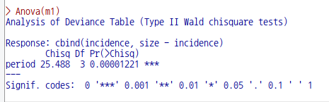
m1 <- glmer(cbind(incidence, size - incidence) ~ period + (1 | herd),
             family = binomial, data = cbpp)
summary(m1)
Anova(m1)
Linux 사례 (MX 21) - R MarkdownLinux 사례 (MX 21)
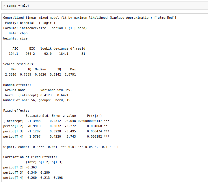
m1p <- glmer(incidence / size ~ period + (1 | herd), weights = size,
             family = binomial, data = cbpp)
summary(m1p)
Anova(m1p)
Linux 사례 (MX 21) - R MarkdownLinux 사례 (MX 21)
## GLMM with individual-level variability (accounting for overdispersion)
cbpp$obs <- 1:nrow(cbpp)
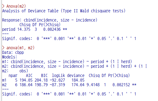
m2 <- glmer(cbind(incidence, size - incidence) ~ period + (1 | herd) + (1|obs),
family = binomial, data = cbpp)
summary(m2)
Anova(m2)
anova(m1, m2)
그리고 '데이터 > 패키지에 있는 데이터 > 첨부된 패키지에서 데이터셋 읽기...' 메뉴 기능을 선택하면 하위 선택 창으로 이동한다. 아래와 같이 lme4 패키지를 선택하고, cbpp 데이터셋을 찾아서 선택한다.
Linux 사례 (MX 21)
cbpp 데이터셋이 활성화된다. R Commander 상단의 메뉴에서 < 활성 데이터셋 없음> 이 'cbpp'로 바뀐다.
summary(cbpp)
str(cbpp)
'통계 > 요약 > 활성 데이터셋' 메뉴 기능을 통해서 cbpp 데이터의 요약 정보를 살펴보자. str() 함수를 이용하여 cbpp 데이터셋의 내부 구조를 살펴보자.
Linux 사례 (MX 21)Linux 사례 (MX 21)
cbpp {lme4}
R Documentation
Contagious bovine pleuropneumonia
Description
Contagious bovine pleuropneumonia (CBPP) is a major disease of cattle in Africa, caused by a mycoplasma. This dataset describes the serological incidence of CBPP in zebu cattle during a follow-up survey implemented in 15 commercial herds located in the Boji district of Ethiopia. The goal of the survey was to study the within-herd spread of CBPP in newly infected herds. Blood samples were quarterly collected from all animals of these herds to determine their CBPP status. These data were used to compute the serological incidence of CBPP (new cases occurring during a given time period). Some data are missing (lost to follow-up).
Format
A data frame with 56 observations on the following 4 variables.
herd
A factor identifying the herd (1 to 15).
incidence
The number of new serological cases for a given herd and time period.
size
A numeric vector describing herd size at the beginning of a given time period.
period
A factor with levels 1 to 4.
Details
Serological status was determined using a competitive enzyme-linked immuno-sorbent assay (cELISA).
Source
Lesnoff, M., Laval, G., Bonnet, P., Abdicho, S., Workalemahu, A., Kifle, D., Peyraud, A., Lancelot, R., Thiaucourt, F. (2004) Within-herd spread of contagious bovine pleuropneumonia in Ethiopian highlands. Preventive Veterinary Medicine 64, 27–40.
Examples
## response as a matrix
(m1 <- glmer(cbind(incidence, size - incidence) ~ period + (1 | herd),
             family = binomial, data = cbpp))
## response as a vector of probabilities and usage of argument "weights"
m1p <- glmer(incidence / size ~ period + (1 | herd), weights = size,
             family = binomial, data = cbpp)
## Confirm that these are equivalent:
stopifnot(all.equal(fixef(m1), fixef(m1p), tolerance = 1e-5),
          all.equal(ranef(m1), ranef(m1p), tolerance = 1e-5))


## GLMM with individual-level variability (accounting for overdispersion)
cbpp$obs <- 1:nrow(cbpp)
(m2 <- glmer(cbind(incidence, size - incidence) ~ period + (1 | herd) +  (1|obs),
              family = binomial, data = cbpp))
'데이터 > 패키지에 있는 데이터 > 첨부된 패키지에서 데이터셋 읽기...' 메뉴 기능을 선택하면 하위 선택 창으로 이동한다. 아래와 같이 carData 패키지를 선택하고, Chile 데이터셋을 찾아서 선택한다.
Linux 사례 (MX 21)
Chile 데이터셋이 활성화된다. R Commander 상단의 메뉴에서 < 활성 데이터셋 없음> 이 'Chile'로 바뀐다.
summary(Chile)
str(Chile)
'통계 > 요약 > 활성 데이터셋' 메뉴 기능을 통해서 Chile 데이터의 요약 정보를 살펴보자. str() 함수를 이용하여 Chile 데이터셋의 내부 구조를 살펴보자.
Linux 사례 (MX 21)
데이터셋의 내부는 다음과 같다:
Linux 사례 (MX 21)
Chile {carData}
R Documentation
Voting Intentions in the 1988 Chilean Plebiscite
Description
The Chile data frame has 2700 rows and 8 columns. The data are from a national survey conducted in April and May of 1988 by FLACSO/Chile. There are some missing data.
Usage
Chile
Format
This data frame contains the following columns:
region
A factor with levels: C, Central; M, Metropolitan Santiago area; N, North; S, South; SA, city of Santiago.
population
Population size of respondent's community.
sex
A factor with levels: F, female; M, male.
age
in years.
education
A factor with levels (note: out of order): P, Primary; PS, Post-secondary; S, Secondary.
income
Monthly income, in Pesos.
statusquo
Scale of support for the status-quo.
vote
a factor with levels: A, will abstain; N, will vote no (against Pinochet); U, undecided; Y, will vote yes (for Pinochet).
Source
Personal communication from FLACSO/Chile.
References
Fox, J. (2016) Applied Regression Analysis and Generalized Linear Models, Third Edition. Sage.
Fox, J. and Weisberg, S. (2019) An R Companion to Applied Regression, Third Edition, Sage.
?swiss  # swiss 데이터셋 도움말 보기

# 아래는 example(swiss) 입니다.

require(stats); require(graphics)
pairs(swiss, panel = panel.smooth, main = "swiss data",
      col = 3 + (swiss$Catholic > 50))
summary(lm(Fertility ~ . , data = swiss))
linux 사례 (MX 21)
pairs(swiss, panel = panel.smooth, main = "swiss data",
      col = 3 + (swiss$Catholic > 50))

pairs(swiss, panel = panel.smooth, main = "swiss data")  # 두 그래프를 비교해 보기
Linux 사례 (MX 21)Linux 사례 (MX 21)
LinearModel.1 <- lm(Fertility ~ . , data = swiss)
summary(LinearModel.1)