모델 > 수치적 진단 > Durbin-Watson 자기상관 검정...
Models > Numerical dignostics > Durbin-Watson test for autocorrelation...

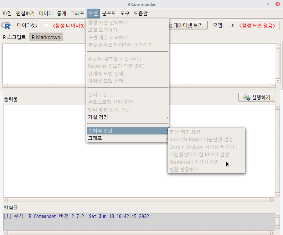
데이터셋을 활성화시키고, 분석 모형을 만들었다면, '모델 > 수치적 진단 > Durbin-Watson 자기상관 검정...' 메뉴 기능을 사용할 수 있다. carData 패키지의 Prestige 데이터셋을 이용하여 연습해보자.
먼저, Prestige 데이터셋을 활성화 시키자. '데이터 > 패키지에 있는 데이터 >
첨부된 패키지에서 데이터셋 읽기...' 메뉴 기능을 선택하고, 다음 화면에서 carData 패키지에 포함된 데이터셋들 중에서 Prestige를 찾아서 선택한다. 그러면, R Commander 상단의 <활성 데이터셋 없음> 버튼이 'Prestige'로 바뀐다.
Prestige 데이터셋을 이용하여 LinearModel.1 모형을 만든다. '통계 > 적합성 모델 > 선형 모델...' 메뉴 기능을 이용할 수 있다.
LinearModel.1 <- lm(prestige ~ education + log(income), data=Prestige)
summary(LinearModel.1)
LinearModel.1 모형이 활성화된 이후, '모델 > 수치적 진단 > Durbin-Watson 자기상관 검정...' 메뉴 기능을 선택하면 아래와 같은 하위 화면이 등장한다. 메뉴 창 오른쪽 끝 아래에 있는 예(OK) 버튼을 누른다.


?dwtest # Durbin Watson 검정 도움말 보기'Models > Numerical diagnostics' 카테고리의 다른 글
| 4. RESET test for nonlinearity... (0) | 2022.06.20 |
|---|---|
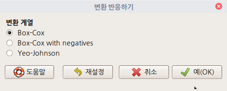
| 6. Response transformation... (0) | 2022.06.20 |
| 5. Bonferroni outlier test (0) | 2022.06.18 |
| 1. Variance-inflation factors (0) | 2022.06.14 |