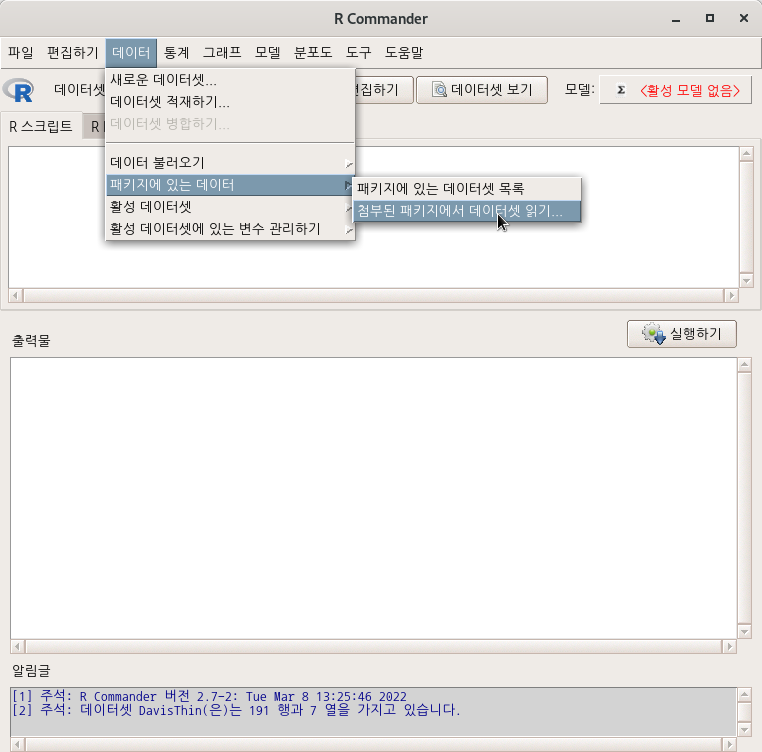
R Commander 화면 상단에서 <데이터셋 보기> 버튼을 누르면 아래와 같은 내부 구성을 확인할 수 있다.
Linux 사례 (MX 21)
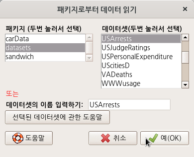
help("USArrests")
USArrests {datasets}
R Documentation
Violent Crime Rates by US State
Description
This data set contains statistics, in arrests per 100,000 residents for assault, murder, and rape in each of the 50 US states in 1973. Also given is the percent of the population living in urban areas.
Usage
USArrests
Format
A data frame with 50 observations on 4 variables.
[,1]
Murder
numeric
Murder arrests (per 100,000)
[,2]
Assault
numeric
Assault arrests (per 100,000)
[,3]
UrbanPop
numeric
Percent urban population
[,4]
Rape
numeric
Rape arrests (per 100,000)
Note
USArrestscontains the data as in McNeil's monograph. For theUrbanPoppercentages, a review of the table (No. 21) in the Statistical Abstracts 1975 reveals a transcription error for Maryland (and that McNeil used the same “round to even” rule thatR'sround()uses), as found by Daniel S Coven (Arizona).
See the example below on how to correct the error and improve accuracy for the ‘<n>.5’ percentages.
Source
World Almanac and Book of facts 1975. (Crime rates).
TheMooredata frame has 45 rows and 4 columns. The data are for subjects in a social-psychological experiment, who were faced with manipulated disagreement from a partner of either of low or high status. The subjects could either conform to the partner's judgment or stick with their own judgment.
Usage
Moore
Format
This data frame contains the following columns:
partner.status
Partner's status. A factor with levels:high,low.
conformity
Number of conforming responses in 40 critical trials.
fcategory
F-Scale Categorized. A factor with levels (note levels out of order):high,low,medium.
fscore
Authoritarianism: F-Scale score.
Source
Moore, J. C., Jr. and Krupat, E. (1971) Relationship between source status, authoritarianism and conformity in a social setting.Sociometry34, 122–134.
Personal communication from J. Moore, Department of Sociology, York University.
References
Fox, J. (2016)Applied Regression Analysis and Generalized Linear Models, Third Edition. Sage.
Fox, J. and Weisberg, S. (2019)An R Companion to Applied Regression, Third Edition, Sage.
TheDavisThindata frame has 191 rows and 7 columns. This is part of a larger dataset for a study of eating disorders. The seven variables in the data frame comprise a "drive for thinness" scale, to be formed by summing the items.
Usage
DavisThin
Format
This data frame contains the following columns:
DT1
a numeric vector
DT2
a numeric vector
DT3
a numeric vector
DT4
a numeric vector
DT5
a numeric vector
DT6
a numeric vector
DT7
a numeric vector
Source
Davis, C., G. Claridge, and D. Cerullo (1997) Personality factors predisposing to weight preoccupation: A continuum approach to the association between eating disorders and personality disorders.Journal of Psychiatric Research31, 467–480. [personal communication from the authors.]
References
Fox, J. and Weisberg, S. (2019)An R Companion to Applied Regression, Third Edition, Sage.
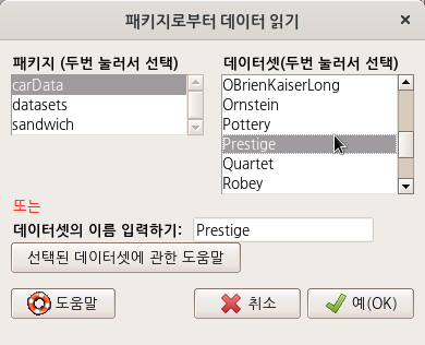
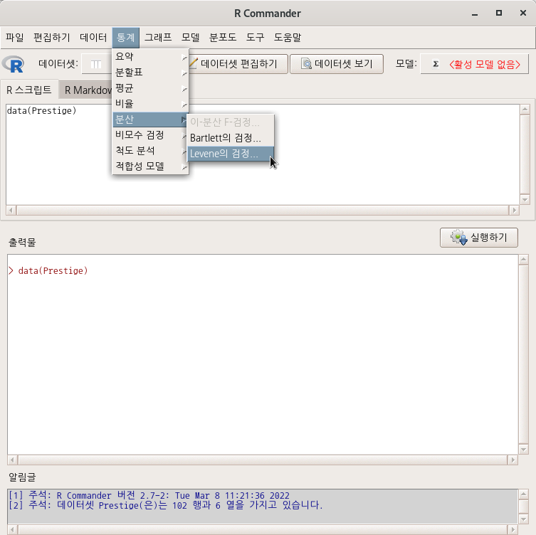
carData 패키지에서 제공하는 Prestige 데이터셋을 활성화 시키자. Prestige 데이터셋에는 type 이라는 세개의 수준을 가진 요인형 변수가 있다. 그 수준 이름은 bc, prof, wc 이다. 직업유형(type)별로 사회적인 권위가 다른지를 확인하는 문제의식이 있다고 하자. 집단별(직업유형, type)로 직업의 사회적 권위(prestige)에 대한 분산의 차이가 있는지를 통계적으로 살펴본다. <중앙(센터)>에서 중앙값과 평균을 선택할 수 있다. 중앙값이 기본 설정이다.
Linux 사례 (MX 21)
Tapply(prestige ~ type, var, na.action=na.omit, data=Prestige) # variances by group
leveneTest(prestige ~ type, data=Prestige, center="median")