모델 > 가설 검정 > 두 모델 비교하기...

Models > Hypothesis test > Compare two models...

Linux 사례 (MX 21)

하나의 데이터셋을 대상으로 가장 최적의 분석모형을 찾고자 할 때, 또는 보다 정교한 설명을 위하여 만들어진 모형들을 비교하고자 할 때 사용하는 기능이다.


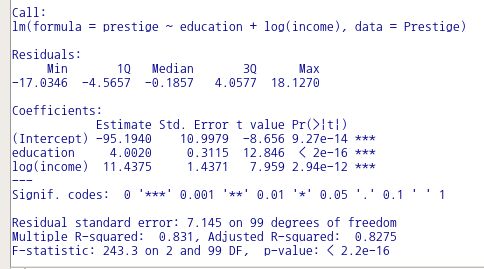
예를 들어, carData에 포함된 Prestige 데이터셋을 이용하여 연습해보자. 직업의 사회적 권위(prestige)에 영향을 미치는 두 개의 독립변수(설명변수)를 교육기간(education)과 수입(income)이라고 가정하자. 그런데 education과 income의 선형적 관계에 대한 보다 깊은 고민을 한다고 생각해보자. education과 income이 서로 독립적인 선형관계로 prestige에 영향을 줄 수도 있고, 또 education과 income이 독립적인 영향을 줄 뿐 만 아니라, 서로 상호작용을 일으키면서 prestige에 영향을 추가 할 수 도 있다고 주장할 수 있다. 이러한 문제의식에서 아래와 같은 두개의 모형을 만들고 또 이 두개의 모형 중에서 어느것이 더 정교한지를 찾는다고 생각해보자.


참고로 연산자 +는 설명변수들의 독립적 선형관계를, *는 독립적 선형관계와 결합적 선형관계를 함께 계산하는데 사용한다.

data(Prestige)   #Prestige 데이터셋 불러오기
LinearModel.1 <- lm(prestige ~ education + income, data=Prestige #변수들의 독립영향 점검
summary(LinearModel.1)
LinearModel.2 <- lm(prestige ~ education*income, data=Prestige)  #변수들의 독립영향 + 결합영향 점검
summary(LinearModel.2)
anova(LinearModel.1, LinearModel.2 #LinearModel.1과 LinearModel.2를 비교하기

Linux 사례 (MX 21)

LinearModel.1과 LinearModel.2라는 두 개의 모형을 만들고 두 개의 모델을 비교하는 방법이다. 모델 > 가설 검정 > 두 모델 비교하기...의 메뉴를 선택하면, 만들어 놓은 두 개의 모형을 비교하는 기능을 이용할 수 있다. 직관적으로 두개의 모형을 차례로 선택해보자. 그리고 예(OK) 버튼을 누른다.

Linux 사례 (MX 21)

R Commander 출력창에 다음과 같은 결과가 출력될 것이다. 출력 내용은 모델 1과 모델 2의 차이가 유의미하며 (Pr(>F)), 모델 2가 보다 설명력이 높다(Sum of sq > 0 또는 RSS < 0)는 뜻으로 해석할 수 있다.

'Models > Hypothesis test' 카테고리의 다른 글

1. ANOVA table...  (0) 2022.03.09

모델 > 관찰 통계를 데이터에 추가하기...

Models > Add observation statistics to data...

Linux 사례 (MX 21)

데이터셋을 활성화시킨 다음, 그 데이터셋으로 모델을 만들었다고 생각하자. 예를 들어, carData 패키지의 Prestige 데이터셋으로 선형 모델을 만들었고, 그 모델을 LinearModel.1이라고 하자.

그럼, R Commander의 화면 메뉴 기능에서 '모델 > 관찰 통계를 데이터에 추가하기...' 기능이 활성화된다. 해당 메뉴 기능을 선택하면 아래와 같은 선택 창이 등장한다. 이 통계치들은 lm() 함수를 이용하여 모델을 생성하는 과정에서 함께 연산된 값들이며, 이 값들을 Prestige 데이터셋에 추가할 것인가를 질문받게 된다.

Linux 사례 (MX 21)

R Commander 화면에서 <데이터셋 보기>를 선택하면 관찰 통계치가 추가되어 있음을 아래와 같이 알 수 있다:

Linux 사례(MX 21)

data(Prestige)         # 데이터셋 불러오기
summary(LinearModel.1) # 모델 만든후 요약정보 보기
Prestige<- within(Prestige, {
  fitted.LinearModel.1 <- fitted(LinearModel.1)
  residuals.LinearModel.1 <- residuals(LinearModel.1)
  rstudent.LinearModel.1 <- rstudent(LinearModel.1)
  hatvalues.LinearModel.1 <- hatvalues(LinearModel.1)
  cooks.distance.LinearModel.1 <- cooks.distance(LinearModel.1)
  obsNumber <- 1:nrow(Prestige) 
})

그래프 > 이산형 수치 변수 그리기...

Graphs > Plot discrete numeric variable...

Linux 사례 (MX 21)

carData 패키지의 Cowles 데이터셋을 활용해서 연습해보자.

data(Cowles, package="carData") # Cowles 데이터셋 불러오기
summary(Cowles)                 # Cowles 데이터셋의 요약정보 보기 (변수이름, 사례요약)

외향성을 의미하는 이산형 수치 변수인 extraversion을 선택한다.

Linux 사례 (MX 21)

요인형 변수 목록에 sex와 volunteer가 있다. volunteer를 선택한다.

Linux 사례 (MX 21)

<선택기능> 창의 선택 기능중에서 <축 크기조정>에 '백분율"을 선택한다. 그리고 <그림 이름표>에는 내용적 이해를 돕는 사항들을 넣을 수 있다.

Linux 사례 (MX 21)

아래와 같이 그래픽 창에 '이산형 수치 변수' extraversion의 백분율 분포가 자원봉사 지원 여부인 volunteer 변수의 요인형 수준인 'no', 'yes' 별로 그래프화된다.

Linux 사례 (MX 21)

with(Cowles, discretePlot(extraversion, by=volunteer, scale="percent", xlab="외향성 (extraversion)",
   ylab="비율 (%)", main="자원봉사 지원여부 그룹에 따른 외향성 분포"))

<관련 사항>

- Cowles 데이터셋 이해하기 -> https://rcmdr.tistory.com/154


Cowles 데이터셋

carData > Cowles data(Cowles, package="carData") help("Cowles") Cowles {carData} R Documentation Cowles and Davis's Data on Volunteering Description The Cowles data frame has 1421 rows and 4 co..

rcmdr.kr


?discretePlot  # RcmdrMisc 패키지의 discretePlot 도움말 보기

if (require(datasets)){
  data(mtcars)
  mtcars$cyl <- factor(mtcars$cyl)
  with(mtcars, {
    discretePlot(carb)
    discretePlot(carb, scale="percent")
    discretePlot(carb, by=cyl)
  })
}

carData::Adler

Linux 사례 (MX 21)

데이터 > 패키지에 있는 데이터 > 첨부된 패키지에서 데이터셋 읽기... 기능을 선택하면, 위와 같은 메뉴 창을 보게된다.

carData를 선택하여 두번 클릭하면, 오른쪽에 carData 패키지에 내장된 데이터셋 목록이 등장한다. Adler 데이터셋을 선택한다.

Linux 사례 (MX 21)

data(Adler, package="carData")  # Adler 데이터셋 활성화시키기
help("Adler", package="carData")# 도움말파일 열기

Linux사례 (MX 21)


Adler {carData} R Documentation

Experimenter Expectations

Description

The Adler data frame has 108 rows and 3 columns.

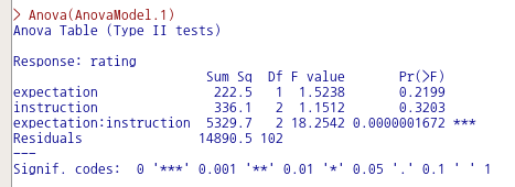
The “experimenters” were the actual subjects of the study. They collected ratings of the apparent success of people in pictures who were pre-selected for their average appearance of success. The experimenters were told prior to collecting data that particular subjects were either high or low in their tendency to rate appearance of success, and were instructed to get good data, scientific data, or were given no such instruction. Each experimenter collected ratings from 18 randomly assigned subjects. This version of the Adler data is taken from Erickson and Nosanchuk (1977). The data described in the original source, Adler (1973), have a more complex structure.

Usage

Adler

Format

This data frame contains the following columns:

instruction

a factor with levels: good, good data; none, no stress; scientific, scientific data.

expectation

a factor with levels: high, expect high ratings; low, expect low ratings.

rating

The average rating obtained.

Source

Erickson, B. H., and Nosanchuk, T. A. (1977) Understanding Data. McGraw-Hill Ryerson.

References

Adler, N. E. (1973) Impact of prior sets given experimenters and subjects on the experimenter expectancy effect. Sociometry 36, 113–126.

통계 > 평균 > 다원 분산 분석...
Statistics > Means > Multi-way ANOVA...

Linux 사례 (MX 21)

다중 분산 분석 (Multi-way ANOVA)은 두개 이상의 요인형 변수들의 작용으로 하나의 수치형 변수에 영향을 주었는가를 점검하는 통계기법이다.

Linux 사례 (MX 21)

data(Adler, package="carData")
help("Adler", package="carData")
AnovaModel.1 <- lm(rating ~ expectation*instruction, data=Adler, contrasts=list(expectation 
  ="contr.Sum", instruction ="contr.Sum"))
Anova(AnovaModel.1)
Tapply(rating ~ expectation + instruction, mean, na.action=na.omit, data=Adler) # means
Tapply(rating ~ expectation + instruction, sd, na.action=na.omit, data=Adler) # std. deviations
xtabs(~ expectation + instruction, data=Adler) # counts

Linux 사례 (MX 21)


?Anova  # car패키지의 Anova 도움말 보기

## Two-Way Anova

mod <- lm(conformity ~ fcategory*partner.status, data=Moore,
  contrasts=list(fcategory=contr.sum, partner.status=contr.sum))
Anova(mod)
Anova(mod, type=3)  # note use of contr.sum in call to lm()

## One-Way MANOVA
## See ?Pottery for a description of the data set used in this example.

summary(Anova(lm(cbind(Al, Fe, Mg, Ca, Na) ~ Site, data=Pottery)))

## MANOVA for a randomized block design (example courtesy of Michael Friendly:
##  See ?Soils for description of the data set)

soils.mod <- lm(cbind(pH,N,Dens,P,Ca,Mg,K,Na,Conduc) ~ Block + Contour*Depth,
    data=Soils)
Manova(soils.mod)
summary(Anova(soils.mod), univariate=TRUE, multivariate=FALSE,
    p.adjust.method=TRUE)

## a multivariate linear model for repeated-measures data
## See ?OBrienKaiser for a description of the data set used in this example.

phase <- factor(rep(c("pretest", "posttest", "followup"), c(5, 5, 5)),
    levels=c("pretest", "posttest", "followup"))
hour <- ordered(rep(1:5, 3))
idata <- data.frame(phase, hour)
idata

mod.ok <- lm(cbind(pre.1, pre.2, pre.3, pre.4, pre.5,
                     post.1, post.2, post.3, post.4, post.5,
                     fup.1, fup.2, fup.3, fup.4, fup.5) ~  treatment*gender,
                data=OBrienKaiser)
(av.ok <- Anova(mod.ok, idata=idata, idesign=~phase*hour))

summary(av.ok, multivariate=FALSE)

## A "doubly multivariate" design with two  distinct repeated-measures variables
## (example courtesy of Michael Friendly)
## See ?WeightLoss for a description of the dataset.

imatrix <- matrix(c(
	1,0,-1, 1, 0, 0,
	1,0, 0,-2, 0, 0,
	1,0, 1, 1, 0, 0,
	0,1, 0, 0,-1, 1,
	0,1, 0, 0, 0,-2,
	0,1, 0, 0, 1, 1), 6, 6, byrow=TRUE)
colnames(imatrix) <- c("WL", "SE", "WL.L", "WL.Q", "SE.L", "SE.Q")
rownames(imatrix) <- colnames(WeightLoss)[-1]
(imatrix <- list(measure=imatrix[,1:2], month=imatrix[,3:6]))
contrasts(WeightLoss$group) <- matrix(c(-2,1,1, 0,-1,1), ncol=2)
(wl.mod<-lm(cbind(wl1, wl2, wl3, se1, se2, se3)~group, data=WeightLoss))
Anova(wl.mod, imatrix=imatrix, test="Roy")

## mixed-effects models examples:

## Not run: 
	library(nlme)
	example(lme)
	Anova(fm2)

## End(Not run)

## Not run: 
	library(lme4)
	example(glmer)
	Anova(gm1)

## End(Not run)

'Statistics > Means' 카테고리의 다른 글

7. Two-factor repeated-measures ANOVA/ANCOVA  (0) 2022.06.30
6. One-factor repeated-measures ANOVA/ANCOVA...  (0) 2022.06.23
4. One-way ANOVA...  (0) 2022.03.07
3. Paired t-test...  (0) 2022.03.07
2. Independent samples t-test...  (0) 2022.03.07

 모델 > 모델 계수 비교하기...

Models > Compare model coefficients...

Linux 사례 (MX 21)

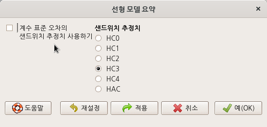
두개 이상의 모델을 선택하고 그 안에 포함된 계수(coefficients)를 비교하는 기능이다.


carData 패키지에 있는 Prestige 데이터셋을 이용하여 income(연수입)과 education(교육연수)가 prestige(직업의 사회적 권위)에 미치는 영향에 대하여 분석한다고 가정하자. 최적의 모델을 찾기 위해서는 먼저 여러개의 모델을 만들어야 한다. 이 경우, 만들어진 여러개의 모델을 비교하는 과정에서 영향력이 통계적으로 지지되는 변수들을 찾고 또 그 계수에 대한 꼼꼼한 점검을 해야하는 경우가 많다.

Linux 사례 (MX 21)

compareCoefs(RegModel.1, RegModel.2)

Linux 사례 (MX 21)

모델 세개를 선택해보자.

Linux 사례 (MX 21)

compareCoefs(LinearModel.3, LinearModel.4, LinearModel.5)

Linux 사례 (MX 21)

모델의 계수를 비교하는 과정에서, 설명변수가 반응변수에 영향을 미치는가에 대한 통계적인 근거를 찾게된다. zvals, pvals, se 등의 인자에 대한 사용을 통하여 보다 정교한 비교 결과를 만들 수 있다.

compareCoefs(RegModel.1, RegModel.2, zvals=TRUE, pvals=TRUE)

Linux 사례 (MX 21)

모델 > 모델 요약하기

Models > Summarize model

Linux 요약 (MX 21)

모델을 만들고, 모델의 요약 정보를 확인할 때 일반적으로 summary() 함수를 사용한다.

carData 패키지의 Prestige 데이터셋으로 선형회귀, 선형모델을 만들었다고 하자. 이 과정에서 다음 사례와 같은 요약 정보가 생산된다:

summary(LinearModel.2)

Linux 사례(MX 21)

여러개의 모델이 있고, 특정 모델의 요약정보를 다시 확인하고자 할 때 사용하는 기능이다.

Linux 사례 (MX 21)

<계수 표준 오차의 샌드위치 추정치 사용하기>에 선택이 되어 있는 경우는 summary() 함수 대신 summarySandwich() 함수가 사용된다.

Linux 사례 (MX 21)

summarySandwich(LinearModel.2, type="hc3")

Linux 사례 (MX 21)

모델 > 활성 모델 선택하기...

Models > Select active model...

Linux 사례 (MX 21)

R Commander 상단에는 메뉴 목록이 있다. 오른쪽 끝부분에 <모델: 모델이름>이 활성화되면 데이터셋으로 분석 모델을 만들었다는 의미가 된다. 그런데, 여러개의 모델을 만들면서 다양한 각도로 분석적 통찰력을 키우는 경우가 일반적이다. R Commander에서는 분석과정에서 만들어진 여러개의 모델을 메모리에 상주시키고, 상황에 맞게 활용할 준비를 갖춘다. 아래의 명령문 프롬프트 창은 세개의 모델이 있음을 알린다. carData 패키지의 Prestige 데이터셋을 이용하여, 선형회귀, 선형모델 기법을 통하여 education(교육연수), income(연소득)이 prestige(직업의 사회적 권위)에 어떤 영향을 미치는가, 또 직업유형별로 차이가 있는가를 분석한다고 가정하자.

data(Prestige, package="carData") # prestige 데이터셋 불러오기
RegModel.1 <- lm(prestige~education+income, data=Prestige) # 선형회귀모델1
summary(RegModel.1)
LinearModel.2 <- lm(prestige ~ education + log(income), data=Prestige)# 선형모델1
summary(LinearModel.2)
LinearModel.4 <- lm(prestige ~ (education + log(income))*type, data=Prestige)# 선형모델2
summary(LinearModel.4)

<활성 모델 선택하기...>기능을 선택하면 아래와 같은 모델 목록창이 등장한다. 목록에서 하나를 선택한다.

Linux 사례 (MX 21)


통계 > 비율 > 일-표본 비율 검정...

Statistics > Proportions > Single-sample proportion test...

Linux 사례 (MX 21)

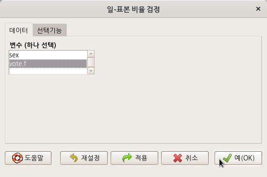
요인형 변수를 두개 이상 가지고 있는 데이터셋이 활성화되어 있다면, '통계 > 비율 > 이-표본 비율 검정..' 메뉴 기능을 이용할 수 있다. carData 패키지에 있는 Chile 데이터셋을 활용해서 연습해보자. 먼저, '데이터 > 패키지에 있는 데이터 > 첨부된 패키지에서 데이터셋 읽기...' 메뉴 기능을 통하여 Chile 데이터셋을 활성화시키자. R Commander 상단에 'Chile'라는 데이터셋이 활성화되었는지 확인하자.


https://rcmdr.tistory.com/239


Chile 데이터셋

carData::Chile() data(Chile, package="carData") '데이터 > 패키지에 있는 데이터 > 첨부된 패키지에서 데이터셋 읽기...' 메뉴 기능을 선택하면 하위 선택 창으로 이동한다. 아래와 같이 carData 패키지를 선택.

rcmdr.kr

요인형 변수 vote를 변형시켜 vote.f 변수를 새롭게 코딩하고 사용하도록 하자.

data(Chile, package="carData")
Chile <- within(Chile, {
  vote.f <- Recode(vote, '"Y" = "yes"; "N" = "no"; else = NA', as.factor=TRUE)
})

Linux 사례 (MX 21)

<선택기능> 창에 표시되어 있는 기본 설정을 그대로 사용하자.

Linux 사례 (MX 21)

local({
  .Table <- xtabs(~ vote.f , data= Chile )
  cat("\nFrequency counts (test is for first level):\n")
  print(.Table)
  prop.test(rbind(.Table), alternative='two.sided', p=.5, conf.level=.95, correct=FALSE)
})

출력창에 나오는 결과는 아래와 같다:

Linux 사례 (MX 21)


?prop.test  # stats 패키지의 prop.test 도움말 보기

heads <- rbinom(1, size = 100, prob = .5)
prop.test(heads, 100)          # continuity correction TRUE by default
prop.test(heads, 100, correct = FALSE)

## Data from Fleiss (1981), p. 139.
## H0: The null hypothesis is that the four populations from which
##     the patients were drawn have the same true proportion of smokers.
## A:  The alternative is that this proportion is different in at
##     least one of the populations.

smokers  <- c( 83, 90, 129, 70 )
patients <- c( 86, 93, 136, 82 )
prop.test(smokers, patients)

https://rcmdr.tistory.com/53


1. Recode variables...

데이터 > 활성 데이터셋의 변수 관리하기 > 변수를 다시 코딩하기... Data > Manage variables in active data set > Recode variables... 기존 변수를 이용하여 새로운 변수를 만들 수 있다. R Commander에서 이..

rcmdr.kr


'Statistics > Proportions' 카테고리의 다른 글

2. Two-sample proportions test...  (0) 2022.06.30

모델 > 그래프 > 효과 그림...

Models > Graphs > Effect plots...

Linux 사례 (MX 21)

'모델 > 그래프 > 효과 그림...' 기능은 미리 모델이 만들어져야 이용할 수 있다. 만들어진 모델은 아래와 같이 R Commander 상단에서 확인할 수 있다. carData 패키지의 Cowles 데이터셋으로 만든 GLM.1 모델을 활용하는 것이다.

Linux 사례 (MX 21)

<모델 효과 그림(들)> 창 중간에 있는 <예측변수 (하나 이상 선택)> 기능에서 sex, neuroticism, extraversion 세 변수를 모두 선택해보자.

Linux 사례 (MX 21)

plot(allEffects(GLM.1))

Linux 사례 (MX 21)


carData 패키지의 Prestige 데이터셋을 이용하여 연습해보자. 아래와 같이 prestige (직업의 사회적 권위)에 대한 education (교육연수), income (연수입), women (여성 참여율)의 영향력을 type (직업유형)별로 살펴보는 모델을 만들었다고 가정하자.

data(Prestige, package="carData")
LinearModel.1 <- lm(prestige ~ education + income + women + type, data=Prestige)
summary(LinearModel.1)

아래와 같이 LinearModel.1의 요약 정보가 출력될 것이다.

Linux 사례 (MX 21)

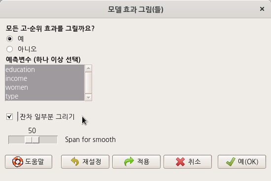
이러한 LinearModel.1의 효과 그림을 시각화 할 수 있다. <모델 효과 그림(들)> 창의 <예측변수(하나 이상 선택)> 기능에서 네개의 변수를 모두 선택해보자. 그리고 예(OK) 버튼을 누른다.

Linux 사례 (MX 21)

plot(allEffects(LinearModel.1))

아래와 같이 그래픽 장치 창에 선택된 변수 네개의 효과 그림이 등장할 것이다.

Linux 사례 (MX 21)

한편, <잔차 일부분 그리기> 기능을 선택해보자. 

Linux 사례 (MX 21)

그래픽 장치 창에 잔차들이 플롯으로 표시된다. 표시된 잔차의 분포를 보면서 추가로로 통찰력을 키울 수 있다.

Linux 사례 (MX 21)

'Models > Graphs' 카테고리의 다른 글

6. Influence index plot...  (0) 2022.06.21
2. Residual quantile-comparison plot...  (0) 2022.06.21
5. Influence plot...  (0) 2022.06.21
4. Added-variable plots...  (0) 2022.06.20
3. Component + residual plots...  (0) 2022.06.20

+ Recent posts