Rcmdr.kr: An R Commander User in Korea

통계 > 적합성 모델 > 선형 회귀...

Statistics > Fit models > Linear regression...

carData 패키지에서 제공하는 Prestige 데이터셋을 불러와서 활성화시키자. 그러면, 위의 화면처럼 <선형 회귀...> 기능이 활성화될 것이다. 이 기능을 선택하면 아래와 같이 Prestige 데이터셋의 변수 목록이 등장하며, 회귀분석을 위한 구조적 설계를 시작한다.

교육연수(education)와 연소득(income)이 직업의 사회적권위(prestige)에 영향을 미치는가? 어떤 영향을 미치는가? 등의 문제의식을 통계적으로 점검한다고 해보자. 교육연수와 연소득은 설명 변수일 것이며, 직업의 사회적 권위는 이 두개의 설명 변수로부터 영향을 받는 반응 변수가 될 것이다. 한편, <모델 이름 입력하기:>에는 RegModel.1이 자동적으로 추천된다. 여러 개의 모델을 만들어 점검하는 경우, 지속적으로 일련번호가 추가된다. 분석가가 자유롭게 모델 이름을 정할 수 있다.

예(OK) 버튼을 누르면, R Commander 화면 상단에 있는 <모델:>옆에 파란색으로 RegModel.1이 등장한다.

RegModel.1 <- lm(prestige~education+income, data=Prestige)

summary(RegModel.1)

R Commander의 출력 창에는 만든 선형 회귀 모델의 결과가 출력된다.

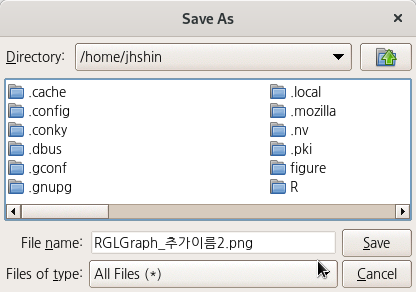
그래프 > 그래프를 파일로 저장하기 > 3차원 RGL 그래프...
Graphs > Save graph to file > 3D RGL graph...

위의 그래프는 carData 패키지에서 제공하는 Prestige 데이터셋을 활용하여 만들었다. 3차원 그래프가 만들어졌다면, <3차원 RGL 그래프...> 기능이 활성화된다. 그리고 그 기능을 마우스로 선택하면 아래와 같은 경로, 파일이름, 형식을 추천하는 메뉴 창이 등장한다.

rgl.snapshot("/home/jhshin/RGLGraph_추가이름2.png")

그래프 > 3D 그래프 > 그래프를 파일로 저장하기
Graphs > 3D graph > Save graph to file

carData 패키지에서 제공하는 Prestige 데이터셋을 활용하여 만든 3차원 산점도이다. 위와 같이 3차원 그래프를 만들었다면, <그래프를 파일로 저장하기> 기능이 활성화될 것이다. 이 기능을 선택하면, 아래와 같이 저장경로와 추천하는 파일이름과 형식이 제공된다.

rgl.snapshot("/home/jhshin/RGLGraph_추가이름1.png")

그래프 > XY 조건 그림...
Graphs > XY conditioning plot...

carData 패키지의 Prestige 데이터셋을 활성화시키자. 연소득과 직업의 사회적귄위에 대한 이해를 확대하고자 income, prestige 변수의 연관성에 대하여 시각적으로 점검한다고 하자. bc, prof, wc라는 수준을 가진 요인형 변수 type을 집단화시켜 시각화에 포함시키자.

<선택기능> 창에 있는 많은 선택 기능은 기본설정으로 놓고 오른쪽의 <그림 이름표>에 그래프의 내용적 이해를 높이고자 관련 사항을 추가적으로 입력하자.

xyplot(prestige ~ income, groups=type, type="p", pch=16, 
  auto.key=list(border=TRUE), par.settings=simpleTheme(pch=16), 
  scales=list(x=list(relation='same'), y=list(relation='same')), data=Prestige, 
  xlab="income (연소득)", ylab="prestige (직업의권위)", main="연소득에 따른 직업의 사회적 권위인식")

그래픽장치 창에 아래와 같은 그래프가 출력된다. 직업유형을 뜻하는 type 변수의 수준인 bc, prof, wc 수준의 범례가 보인다. 그리고 그 색깔별로 점들이 찍혀 있어, 추가적인 이해를 제공한다.

아래 그림은 직업유형 변수인 type을 "Groups 'groups='에서 해제하고, Conditions'|'에 선택한다.

<선택기능>창의 오른쪽에 있는 <그림 이름표>에 내용적인 이해를 높이는 이름표과 제목을 넣자.

xyplot(prestige ~ income | type, type="p", pch=16, auto.key=list(border=TRUE),
   par.settings=simpleTheme(pch=16), scales=list(x=list(relation='same'), 
  y=list(relation='same')), data=Prestige, xlab="income (연소득)", ylab="prestige 
  (직업의권위)", main="연소득에 따른 직업의 사회적 권위의식")

아래에 있는 그래픽장치 창은 위에 있는 그래픽장치 창과 달리 직업유형별(bc, prof, wc)별로 산점도가 각각 제작된다.

xyplot() 함수는 시계열적 수치형 변수와 관련해서는 lineplot()과 유사하게 그래프를 출력할 수 있다. carData 패키지의 Bfox의 사례를 수치형 time 변수로 변환시키고 그래프를 만들어보자.

<선택기능> 창에 있는 <그림 유형(하나 또는 둘 모두)>에 점/줄(선) 모두 선택해보자. 물론 <그림 이름표>에 내용을 추가할 수도 있다.

xyplot(menwage + womwage ~ time, type=c("p", "l"), pch=16, auto.key=list(border=TRUE), 
	par.settings=simpleTheme(pch=16), scales=list(x=list(relation='same'), 
	y=list(relation='same')), data=Bfox)

시간의 흐름에 따른 수치형 변수들의 변화 흐름을 파악할 수 있다. 주의해야할 점은 두개 이상의 수치형 변수를 그래프에 모두 넣을 경우, 각 변수들의 사례 기준(크기, 비율 등)이 동일해야 시각화가 특징을 잡아내는데 효과적이다.

?xyplot  # lattice 패키지의 xyplot 도움말 보기

require(stats)

## Tonga Trench Earthquakes

Depth <- equal.count(quakes$depth, number=8, overlap=.1)
xyplot(lat ~ long | Depth, data = quakes)
update(trellis.last.object(),
       strip = strip.custom(strip.names = TRUE, strip.levels = TRUE),
       par.strip.text = list(cex = 0.75),
       aspect = "iso")

## Examples with data from `Visualizing Data' (Cleveland, 1993) obtained
## from http://cm.bell-labs.com/cm/ms/departments/sia/wsc/

EE <- equal.count(ethanol$E, number=9, overlap=1/4)

## Constructing panel functions on the fly; prepanel
xyplot(NOx ~ C | EE, data = ethanol,
       prepanel = function(x, y) prepanel.loess(x, y, span = 1),
       xlab = "Compression Ratio", ylab = "NOx (micrograms/J)",
       panel = function(x, y) {
           panel.grid(h = -1, v = 2)
           panel.xyplot(x, y)
           panel.loess(x, y, span=1)
       },
       aspect = "xy")

## Extended formula interface 

xyplot(Sepal.Length + Sepal.Width ~ Petal.Length + Petal.Width | Species,
       data = iris, scales = "free", layout = c(2, 2),
       auto.key = list(x = .6, y = .7, corner = c(0, 0)))


## user defined panel functions

states <- data.frame(state.x77,
                     state.name = dimnames(state.x77)[[1]],
                     state.region = state.region)
xyplot(Murder ~ Population | state.region, data = states,
       groups = state.name,
       panel = function(x, y, subscripts, groups) {
           ltext(x = x, y = y, labels = groups[subscripts], cex=1,
                 fontfamily = "HersheySans")
       })

## Stacked bar chart

barchart(yield ~ variety | site, data = barley,
         groups = year, layout = c(1,6), stack = TRUE,
         auto.key = list(space = "right"),
         ylab = "Barley Yield (bushels/acre)",
         scales = list(x = list(rot = 45)))

bwplot(voice.part ~ height, data=singer, xlab="Height (inches)")

dotplot(variety ~ yield | year * site, data=barley)

## Grouped dot plot showing anomaly at Morris

dotplot(variety ~ yield | site, data = barley, groups = year,
        key = simpleKey(levels(barley$year), space = "right"),
        xlab = "Barley Yield (bushels/acre) ",
        aspect=0.5, layout = c(1,6), ylab=NULL)

stripplot(voice.part ~ jitter(height), data = singer, aspect = 1,
          jitter.data = TRUE, xlab = "Height (inches)")

## Interaction Plot

xyplot(decrease ~ treatment, OrchardSprays, groups = rowpos,
       type = "a",
       auto.key =
       list(space = "right", points = FALSE, lines = TRUE))

## longer version with no x-ticks

## Not run: 
bwplot(decrease ~ treatment, OrchardSprays, groups = rowpos,
       panel = "panel.superpose",
       panel.groups = "panel.linejoin",
       xlab = "treatment",
       key = list(lines = Rows(trellis.par.get("superpose.line"),
                  c(1:7, 1)),
                  text = list(lab = as.character(unique(OrchardSprays$rowpos))),
                  columns = 4, title = "Row position"))

## End(Not run)

carData > Bfox

data(Bfox, package="carData")

Bfox 데이터셋이 활성화되었다면, 도움말 기능을 통하여 데이터셋의 정보를 확인할 수 있다.

Canadian Women's Labour-Force Participation

Description

The Bfox data frame has 30 rows and 7 columns. Time-series data on Canadian women's labor-force participation, 1946–1975.

Usage

Bfox

Format

This data frame contains the following columns:

partic

Percent of adult women in the workforce.

tfr

Total fertility rate: expected births to a cohort of 1000 women at current age-specific fertility rates.

menwage

Men's average weekly wages, in constant 1935 dollars and adjusted for current tax rates.

womwage

Women's average weekly wages.

debt

Per-capita consumer debt, in constant dollars.

parttime

Percent of the active workforce working 34 hours per week or less.

Warning

The value of tfr for 1973 is misrecorded as 2931; it should be 1931.

Source

Fox, B. (1980) Women's Domestic Labour and their Involvement in Wage Work. Unpublished doctoral dissertation, p. 449.

References

Fox, J. (2016) Applied Regression Analysis and Generalized Linear Models, Third Edition. Sage.

carData > OBrienKaiserLong

OBrienKaiserLong 데이터셋은 carData 패키지에 포함되어 있다. carData 패키지는 Rcmdr 패키지가 호출될 때 자동으로 함께 호출되기 때문에, OBrienKaiserLong 데이터셋을 R Commander에서 메뉴기능을 통해서 활성데이터셋으로 불러올 수 있다.

https://rcmdr.kr/37

통계> 요약 > 활성 데이터셋 메뉴를 통하여 OBrienKaiserLong  데이터셋의 요약정보를 확인할 수 있다.

summary() 함수를 이용한 것을 알 수 있다.

str() 함수를 활용하여 입력창에 직접 str(OBrienKaiserLong)을 입력하고 실행하여, 출력창에 다음과 같이 OBrienKaiserLong 데이터셋의 구조적 정보도 확인할 수 있다.

R Commander 화면에서 <데이터셋 보기> 버튼을 누르면 다음과 같은 내부 구성을 볼 수 있다:

O'Brien and Kaiser's Repeated-Measures Data in "Long" Format

Description

Contrived repeated-measures data from O'Brien and Kaiser (1985). For details see OBrienKaiser, which is for the "wide" form of the same data.

Usage

OBrienKaiserLong

Format

A data frame with 240 observations on the following 6 variables.

treatment

a between-subjects factor with levels control, A, B.

gender

a between-subjects factor with levels F, M.

score

the numeric response variable.

id

the subject id number.

phase

a within-subjects factor with levels pre, post, fup.

hour

a within-subjects factor with levels 1, 2, 3, 4, 5.

Source

O'Brien, R. G., and Kaiser, M. K. (1985) MANOVA method for analyzing repeated measures designs: An extensive primer. Psychological Bulletin 97, 316–333, Table 7.

See Also

OBrienKaiser.

Examples

head(OBrienKaiserLong, 15) # first subject

carData 패키지에 있는  OBrienKaiser 데이터셋이다. carData 패키지는 Rcmdr 패키지가 호출될 때 자동으로 함께 호출되기 때문에 R Commander에서 carData 패키지에 포함된 데이터셋들을 자유롭게 호출할 수 있다.

https://rcmdr.kr/37

OBrienKaiser 데이터셋은 R Commander에서 활성 데이터셋으로 이용할 수 있다. 그러나 '통계 > 요약 > 활성데이터셋' 기능은 사용할 수 없다. 다음과 같은 오류문을 Rgui 창에서 보게된다.

Error in sprintf(gettextRcmdr("There are %d variables in the data set %s.\nDo you want to proceed?"),  : 
  '%d'는 유효하지 않은 포맷입니다; 문자형 객체들에는 포맷 %s를 사용해주세요

입력창에 str(OBrienKaiser) 함수를 입력하고 실행하여 OBrienKaiser 데이터셋의 구조를 살펴보자.

입력창에 summary(OBrienKaiser) 함수를 입력하고 실행하여 요약 정보를 살펴보자.

O'Brien and Kaiser's Repeated-Measures Data

Description

These contrived repeated-measures data are taken from O'Brien and Kaiser (1985). The data are from an imaginary study in which 16 female and male subjects, who are divided into three treatments, are measured at a pretest, postest, and a follow-up session; during each session, they are measured at five occasions at intervals of one hour. The design, therefore, has two between-subject and two within-subject factors.

The contrasts for the treatment factor are set to -2, 1, 1 and 0, -1, 1. The contrasts for the gender factor are set to contr.sum.

Usage

OBrienKaiser

Format

A data frame with 16 observations on the following 17 variables.

treatment

a factor with levels control A B

gender

a factor with levels F M

pre.1

pretest, hour 1

pre.2

pretest, hour 2

pre.3

pretest, hour 3

pre.4

pretest, hour 4

pre.5

pretest, hour 5

post.1

posttest, hour 1

post.2

posttest, hour 2

post.3

posttest, hour 3

post.4

posttest, hour 4

post.5

posttest, hour 5

fup.1

follow-up, hour 1

fup.2

follow-up, hour 2

fup.3

follow-up, hour 3

fup.4

follow-up, hour 4

fup.5

follow-up, hour 5

Source

O'Brien, R. G., and Kaiser, M. K. (1985) MANOVA method for analyzing repeated measures designs: An extensive primer. Psychological Bulletin 97, 316–333, Table 7.

Examples

OBrienKaiser
contrasts(OBrienKaiser$treatment)
contrasts(OBrienKaiser$gender)

활성 데이터셋에 관한 도움말 (만약 이용가능하다면)

Data > Active data set > Help on active data set (if available)

R에서 이용가능한 많은 패키지에는 예제용 데이터셋이 많이 포함되어 있다. 이러한 예제용 데이터셋은 대부분 도움말을 갖고 있다. 내장된 예제용 데이터셋을 활성 데이터로 불러온 경우는 이 명령을 유용하게 사용할 수 있다.

carData 패키지의 Prestige 데이터셋이 활성화되었다면, 도움말을 볼 수 있다:

help("Prestige")

help(Prestige)

?(Prestige) 등으로 입력창에 직접 입력할 수 도 있다.

help("데이터셋이름")

아래의 참고사항은 Prestige 데이터셋과 유사하게, carData 패키지에 담겨있는 DavisThin 데이터셋이다. 같은 방식으로 연습할 수 있다.

https://rcmdr.tistory.com/141

데이터 > 데이터셋 병합하기...

Data > Merge data sets...

두 개 이상의 데이터셋이 객체로서 메모리에 있는 경우 (R Commander에서 인식하는 경우), Merge data sets...라는 기능을 이용할 수 있다. 데이터셋이 없거나 하나인 경우, 회색의 불활성 메뉴로서 표시된다.

- 행 병합하기는 두개의 데이터셋을 위, 아래로 이어 붙인다.

- 열 병합하기는 두개의 데이터셋을 왼쪽, 오른쪽으로 이어 붙인다.

'행 병합하기'를 하려면 동일한 변수들을 갖고 있어야 하며, '열 병합하기'를 하려면 동일한 사례들을 갖고 있어야 한다.

carData 패키지에 있는 Prestige 데이터셋으로 연습해보자.

https://rcmdr.tistory.com/143

Prestige 데이터셋의 하위셋 Prestige.sub1과 Prestige.sub2 두개를 만들자.

data(Prestige, package="carData")    # Prestige 데이터셋 불러오기
Prestige.sub1 <- Prestige[-c(61:nrow(Prestige)),] 
                                     # Prestige 데이터셋에서 사례 지우기1 (61부터 끝까지)
Prestige.sub2 <- Prestige[-c(1:60),] # Prestige 데이터셋에서 사례 지우기2 (1부터 60까지)

https://rcmdr.tistory.com/48 <- 화면의 메뉴를 이용하여 사례 제거를 연습할 수 있다.

아래의 내용은 Prestige.sub1과 Prestige.sub2를 병합하고자 하는 연습이다. <첫째 데이터셋(하나 선택)>과 <둘째 데이터셋 (하나 선택)>에서 데이터셋을 하나씩 선택하고, 공통의 데이터 구조를 가진 두개의 데이터셋을 이어붙이는 <행 병합하기>의 병합 방향을 선택해보자.

MergedDataset <- mergeRows(Prestige.sub1, Prestige.sub2, common.only=FALSE)

?mergeRows  # RcmdrMisc 패키지의 mergeRows 도움말 보기

if (require(car)){
    data(Duncan)
    D1 <- Duncan[1:20,]
    D2 <- Duncan[21:45,]
    D <- mergeRows(D1, D2)
    print(D)
    dim(D)
}