통계 > 적합성 모델 > 다항 로짓 모델...
Statistics > Fit models > Multinomial logit model...

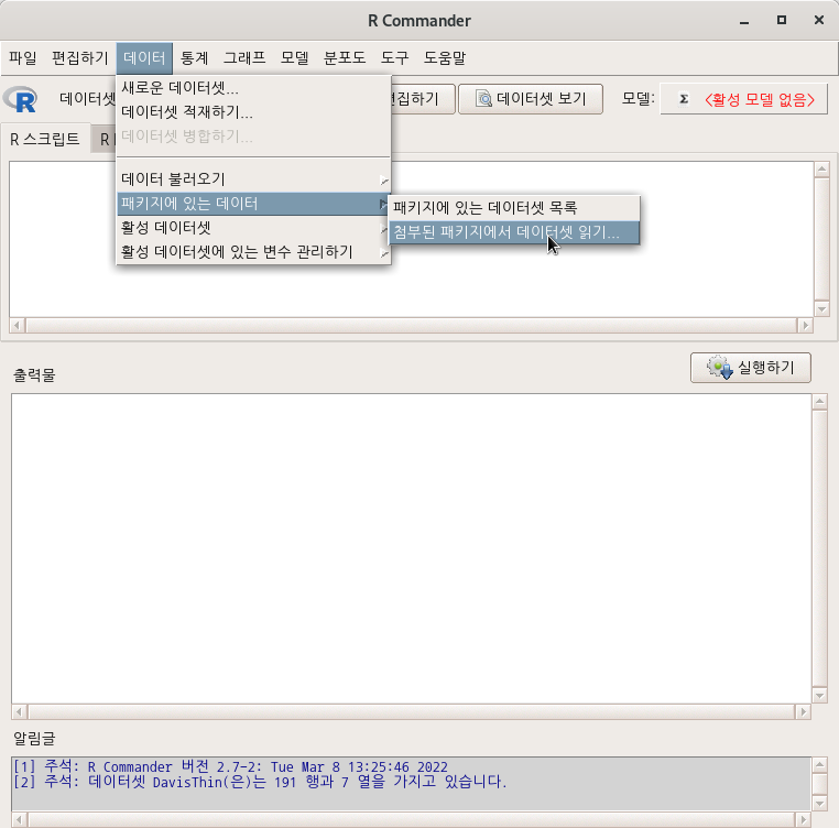
MASS 패키지에 있는 birthwt 데이터셋을 활용해보자. 먼저 birthwt 데이터셋을 활성화 시킨다. https://rcmdr.kr/149
birthwt 데이터셋
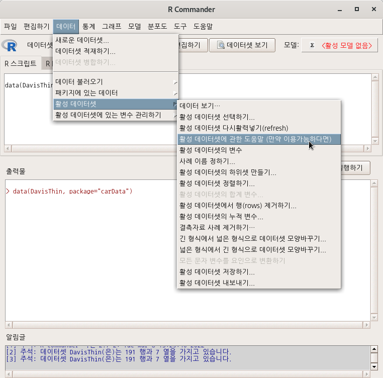
MASS > birthwt data(birthwt, package="MASS") birthwt 데이터셋이 활성화된 후, <데이터셋 보기> 버튼을 누르면 아래와 같이 내부 구성을 볼 수 있다: help("birthwt")
rcmdr.kr
이후 일부 변수의 특징을 변화시켜 bwt라는 새로운 데이터셋을 만들자.아래의 <일반화 선형 모델> 연습 중간에 bwt를 만드는 스크립트가 있다. https://rcmdr.tistory.com/150
3. Generalized linear model...
통계 > 적합성 모델 > 일반화 선형 모델... Statistics > Fit models > Generalized linear model... MASS 패키지에 있는 birthwt 데이터셋을 활용하자. https://rcmdr.tistory.com/149 birthwt data(birthwt, pa..
rcmdr.kr
아래 화면은 bwt 데이터셋을 활용한 사례이다. low 변수를 반응변수로, 다른 나머지 변수를 설명변수군에 모두 포함시키자.

MLM.1 <- multinom(low ~ ., data=bwt, trace=FALSE)
summary(MLM.1, cor=FALSE, Wald=TRUE)
MLM.1 이라는 모형이 만들어졌다면, '모델 > 가설 검정 > 분산분석표...' 메뉴 기능을 이용할 수 있다.

'Statistics > Fit models' 카테고리의 다른 글
| 5. Ordinal regression model... (0) | 2022.06.24 |
|---|---|
| 6. Linear mixed model... (0) | 2022.06.23 |
| 3. Generalized linear model... (0) | 2022.03.09 |
| 2. Linear model... (0) | 2022.03.07 |
| 1. Linear regression... (0) | 2022.03.07 |