Rcmdr.kr: An R Commander User in Korea

통계 > 비모수 검정 > 쌍-표본 Wilcoxon test...

Statistics > Nonparametric tests > Paired-samples Wilcoxon test...

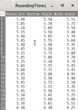
depression 이라는 이름의 데이터셋을 만들자. first, second, change 라는 세개의 변수를 갖는다고 하자. change 변수는 second와 first의 차이를 사례 값으로 갖는다고 하자. 아래와 같을 것이다.

first <- c(1.83,  0.50,  1.62,  2.48, 1.68, 1.88, 1.55, 3.06, 1.30)
second <- c(0.878, 0.647, 0.598, 2.05, 1.06, 1.29, 1.06, 3.14, 1.29)
change <- second - first  # compute new variable 참조할 것
depression <- data.frame(cbind(first, second, change)) # 세개의 vector를 묶어 데이터프레임으로 전환

https://rcmdr.kr/54

<선택기능> 창에 있는 기본 선택 사양을 그대로 사용해보자. <대립 가설>에서 '양쪽(측)'이 선택되어 있다. depression 데이터셋의 second 변수와 first 변수 사이에 순위 차이가 있는가를 살펴보는 것이라 할 수 있다.

with(depression, median(second - first, na.rm=TRUE)) # median difference
with(depression, wilcox.test(second, first, alternative='two.sided', 
  paired=TRUE)) # 양측 검정
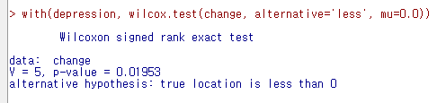
with(depression, wilcox.test(second, first, alternative='less', paired=TRUE))
                # 단측 검정 ( 차이 < 0 )

<선택 기능> 창에서 <대립 가설>에 '차이 < 0'를 선택하자. second 변수의 사례 값이 first 변수의 사례 값보다 작아졌는지를 점검하는 것이다. (depression이 작아졌다는 것은 개선되었다는 의미로 해석될 수도 있다.)

통계 > 비모수 검정 > 일-표본 Wilcoxon 검정...

Statistics > Nonparametric tests > Single-sample Wilcoxon test...

먼저 '통계 > 비모수 검정 > 쌍-표본 Wilcoxon 검정...'을 살펴보는 것을 추천한다. depression 이라는 데이터셋을 만들고, 변수 first, second, change를 만들었다. change는 second와 first의 차이에 관련 사례 값을 갖는다.

https://rcmdr.tistory.com/179

'통계 > 비모수 검정 > 일-표본 Wilcoxon 검정...'은 depression 데이터셋의 change 변수처럼 두 개 변수의 차이를 갖는 (또는 차이가 계산된) 변수를 기준값과 비교하여 차이 검정을 하는 기법이다. 때로는 특정 변수와 기준 값의 비교를 통하여 검정을 하기도 한다.

데이터셋과 변수에 대한 의미적 판단이 깊은 경우 <대립 가설>의 선택을 다양하게 결정할 수 있다. 아래 화면에서 'mu < 0'은 change가 귀무(영) 가설, mu=0.0 일 때 depression 의 변화가 작아졌음을 확인하는 것으로 이해할 수 있다.

with(depression, median(change, na.rm=TRUE))
with(depression, mean(change, na.rm=TRUE))
with(depression, wilcox.test(change, alternative='less', mu=0.0))

출력 창에 아래와 같이 검정의 통계적 정보가 제공된다:

통계 > 비모수 검정 > 이-표본 Wilcoxon 검정...

Statistics > Nonparametric tests > Two-sample Wilcoxon test...

'통계 > 비모수 검정 > 이-표본 Wilcoxon 검정...' 기능을 이용하기 위해서 데이터셋을 선택하고, 정비해보자. datasets 패키지에 있는 airquality 데이터셋을 선택하고, 그 안에 있는 변수 Month 사례 값들 중에서 5월, 8월에 해당하는 5, 8을 선택한 하위 데이터셋을 만들고, airquality.sub라 이름 붙이자. 그리고, 5, 8을 요인화 시켜서, May, August라고 수준을 만들자.

https://rcmdr.kr/100

data(airquality, package="datasets") # airquality 데이터셋 불러오기
airquality.sub <- subset(airquality, subset=Month %in% c(5, 8)) 
                                     # 5월, 8월만 포함하는 하위셋 만들기
summary(airquality.sub)
airquality.sub <- within(airquality.sub, {
  Month.f <- factor(Month, labels=c('May','August'))
})                                   # Month.f라는 요인형 변수 만들기

집단 변수인 Month.f는 두개의 수준을 갖고 있고, 이 두개의 수준을 기준으로 Ozone을 비교하는 것이다.

<선택기능> 창에 있는 기본 설정을 우선 그대로 사용해보자. 향후 데이터셋과 변수에 대한 이해력이 높아지면, 다양한 선택을 할 수 있다.

Tapply(Ozone ~ Month.f, median, na.action=na.omit, data=airquality.sub) 
  # medians by group
wilcox.test(Ozone ~ Month.f, alternative="two.sided", data=airquality.sub)

통계 > 비모수 검정 > Friedman 순위-합 검정...

Statistics > Nonparametric tests > Friedman rank-sum test...

<Friendman 순위-합 검정...> 기능은 두개 이상의 수치형 변수가 데이터셋에 포함되어 있을때 활성화된다. <Friedman 순위-합 검정...> 기능의 함수적 특징을 이해하기 위하여 먼저 아래와 같이 RoundingTimes라는 데이터셋을 만들어보자.

RoundingTimes <-
data.frame(matrix(c(5.40, 5.50, 5.55,
         5.85, 5.70, 5.75,
         5.20, 5.60, 5.50,
         5.55, 5.50, 5.40,
         5.90, 5.85, 5.70,
         5.45, 5.55, 5.60,
         5.40, 5.40, 5.35,
         5.45, 5.50, 5.35,
         5.25, 5.15, 5.00,
          5.85, 5.80, 5.70,
         5.25, 5.20, 5.10,
         5.65, 5.55, 5.45,
         5.60, 5.35, 5.45,
         5.05, 5.00, 4.95,
         5.50, 5.50, 5.40,
         5.45, 5.55, 5.50,
         5.55, 5.55, 5.35,
         5.45, 5.50, 5.55,
         5.50, 5.45, 5.25,
         5.65, 5.60, 5.40,
         5.70, 5.65, 5.55,
         6.30, 6.30, 6.25),
       nrow = 22,
       byrow = TRUE,
       dimnames = list(1 : 22,
                       c("Round Out", "Narrow Angle", "Wide Angle"))))
summary(RoundingTimes)     # RoundingTimes 데이터셋 보기

이 데이터셋을 만드는 이유는 friedman.test()라는 함수의 예제 연습에 포함되어있기 때문이다. RoundingTimes 데이터셋은 아래와 같은 내부 구성을 갖는다:

RoungdingTimes 라는 데이터셋을 만들고, 화면 맨 위에 있는 <Friedman 순위-합 검정...> 기능을 선택하면 추가적인 선택 메뉴 창으로 넘어간다. <Friedman 순위 합 검정> 창에서 <반복-측정 변수 (두개 이상 선택)>에서 세개의 변수를 모두 선택하고, 예(OK) 버튼을 누른다.

local({
  .Responses <- na.omit(with(RoundingTimes, cbind(Narrow.Angle, Round.Out, Wide.Angle)))
  cat("\nMedians:\n") 
  print(apply(.Responses, 2, median)) 
  friedman.test(.Responses)
})

help("friedman.test")     # Friedman 순위 합 검정 도움말 보기
example("friedman.test")  # Friedman 순위 합 검정 예제 연습하기

통계 > 차원 분석 > 군집 분석 > 위계 군집화를 데이터셋에 추가하기...

Statistics > Dimensional Analysis > Cluster Analysis > Add hierarchical clustering to data set...

 ' 통계 > 차원 분석 > 군집 분석 > 위계 군집 분석...' 기능을 진행했다고 하자. 그 다음에 <위계군집화를 데이터 셋에 추가하기...>를 이용할 수 있다. <군집의 수:>를 3으로 변경하자. 그리고 예(OK) 버튼을 누르면, hclus.label라는 변수가 USArrests 데이터셋에 추가된다.

R Commander 상단에 있는 <데이터셋 보기> 버튼을 눌러보자. 아래와 같이 데이터셋의 내부 구성이 보일 것이다. hclus.label 변수가 추가되어 있음을 확인할 수 있다:

통계 > 차원 분석 > 군집 분석 > 위계 군집화 요약하기...

Statistics > Dimensional analysis > Cluster analysis > Summarizing hierarchical clustering...

'통계 > 차원 분석 > 군집 분석 > 위계 군집 분석'을 하였다고 하자. 그 다음에는 <위계 군집화 요약하기...> 기능을 사용할 수 있다.

https://rcmdr.kr/172

<위계적 군집 요약> 창에서 <군집의 수>를 3으로 변경해보자. <군집 요약 인쇄하기>, <군집 행렬도(Bi-plot)> 등이 선택되어 있는 것을 점검하자.

예(OK) 버튼을 누르면, 아래와 같은 그래픽 창이 등장한다.

summary(as.factor(cutree(HClust.1, k = 3))) # Cluster Sizes
by(model.matrix(~-1 + Assault + Murder + Rape + UrbanPop, USArrests), as.factor(cutree(HClust.1, k 
  = 3)), colMeans) # Cluster Centroids
biplot(princomp(model.matrix(~-1 + Assault + Murder + Rape + UrbanPop, USArrests)), xlabs = 
  as.character(cutree(HClust.1, k = 3)))

통계 > 차원 분석 > 군집 분석 > 위계 군집 분석...

Statistics > Dimensional analysis > Cluster analysis > Hierarchical cluster analysis...

datasets 패키지에 있는 USArrests 데이터셋을 활용해서, 위계 군집 분석을 연습해보자. 우선 USArrests 데이터셋을 활성화시킨다.

https://rcmdr.kr/144

<위계적 군집화> 창에서 아래와 같이 변수 네개를 모두 선택한다. 그리고, 기본으로 추천되는 HClust.1를 군집화 이름으로 사용하자. 

<선택기능> 창에서 기본설정된 사항들을 그대로 사용해보자. <군집화 방법>, <거리 측정>, <덴드로그램 그리기> 등을 살펴본다.

예(OK) 버튼을 누르면, 아래와 같은 그래픽 창이 등장한다.

data(USArrests, package="datasets")
HClust.1 <- hclust(dist(model.matrix(~-1 + Assault+Murder+Rape+UrbanPop, USArrests)) , method= 
  "ward")
plot(HClust.1, main= "Cluster Dendrogram for Solution HClust.1", xlab= 
  "Observation Number in Data Set USArrests", sub="Method=ward; Distance=euclidian")

통계 > 차원 분석 > 군집 분석 > k-평균 군집 분석...

Statistics > Dimensional analysis > Cluster analysis > k-means cluster analysis...

datasets 패키지에서 제공하는 USArrests 데이터셋을 이용해보자.

https://rcmdr.tistory.com/144

데이터셋에 포함된 네개의 변수를 모두 선택한다.

<선택기능> 창에서, 군집의 수를 3개, 초기값의 수를 5번으로, 최대 반복 횟수를 5회로 정해보자. 데이터셋에 추가될 변수 이름이 KMeans가 될 것이다. 아래 있는 선택사항에서 데이터셋에 군집 할당하기를 선택한다.

위 화면에서 선택된 군집 행렬도(Bi-plot)이 아래와 같이 생산된다.

USArrests 데이터셋에 변수 KMeans가 추가될 것이다. R Commander 상단에 있는 <데이터셋 보기> 버튼을 눌러보자. KMeans 변수는 요인형으로 1, 2, 3 이라는 세개의 군집을 표시한다.

아래 화면은 다소 복잡해보일 것이다. 그러나 객체 .cluster가 만들어졌으며, 그 객체안에 있는 $size, $withinss, $tot.withinss, $betweenss 등의 정보를 차례를 보여준다고 생각하자.  그리고 biplot을 생산하고, USArrests 데이터셋에 KMeans라는 변수를 추가하는 것이다.

통계 > 평균 > 다원 분산 분석...
Statistics > Means > Multi-way ANOVA...

다중 분산 분석 (Multi-way ANOVA)은 두개 이상의 요인형 변수들의 작용으로 하나의 수치형 변수에 영향을 주었는가를 점검하는 통계기법이다.

data(Adler, package="carData")
help("Adler", package="carData")

AnovaModel.1 <- lm(rating ~ expectation*instruction, data=Adler, contrasts=list(expectation 
  ="contr.Sum", instruction ="contr.Sum"))
Anova(AnovaModel.1)
Tapply(rating ~ expectation + instruction, mean, na.action=na.omit, data=Adler) # means
Tapply(rating ~ expectation + instruction, sd, na.action=na.omit, data=Adler) # std. deviations
xtabs(~ expectation + instruction, data=Adler) # counts

?Anova  # car패키지의 Anova 도움말 보기

## Two-Way Anova

mod <- lm(conformity ~ fcategory*partner.status, data=Moore,
  contrasts=list(fcategory=contr.sum, partner.status=contr.sum))
Anova(mod)
Anova(mod, type=3)  # note use of contr.sum in call to lm()

## One-Way MANOVA
## See ?Pottery for a description of the data set used in this example.

summary(Anova(lm(cbind(Al, Fe, Mg, Ca, Na) ~ Site, data=Pottery)))

## MANOVA for a randomized block design (example courtesy of Michael Friendly:
##  See ?Soils for description of the data set)

soils.mod <- lm(cbind(pH,N,Dens,P,Ca,Mg,K,Na,Conduc) ~ Block + Contour*Depth,
    data=Soils)
Manova(soils.mod)
summary(Anova(soils.mod), univariate=TRUE, multivariate=FALSE,
    p.adjust.method=TRUE)

## a multivariate linear model for repeated-measures data
## See ?OBrienKaiser for a description of the data set used in this example.

phase <- factor(rep(c("pretest", "posttest", "followup"), c(5, 5, 5)),
    levels=c("pretest", "posttest", "followup"))
hour <- ordered(rep(1:5, 3))
idata <- data.frame(phase, hour)
idata

mod.ok <- lm(cbind(pre.1, pre.2, pre.3, pre.4, pre.5,
                     post.1, post.2, post.3, post.4, post.5,
                     fup.1, fup.2, fup.3, fup.4, fup.5) ~  treatment*gender,
                data=OBrienKaiser)
(av.ok <- Anova(mod.ok, idata=idata, idesign=~phase*hour))

summary(av.ok, multivariate=FALSE)

## A "doubly multivariate" design with two  distinct repeated-measures variables
## (example courtesy of Michael Friendly)
## See ?WeightLoss for a description of the dataset.

imatrix <- matrix(c(
	1,0,-1, 1, 0, 0,
	1,0, 0,-2, 0, 0,
	1,0, 1, 1, 0, 0,
	0,1, 0, 0,-1, 1,
	0,1, 0, 0, 0,-2,
	0,1, 0, 0, 1, 1), 6, 6, byrow=TRUE)
colnames(imatrix) <- c("WL", "SE", "WL.L", "WL.Q", "SE.L", "SE.Q")
rownames(imatrix) <- colnames(WeightLoss)[-1]
(imatrix <- list(measure=imatrix[,1:2], month=imatrix[,3:6]))
contrasts(WeightLoss$group) <- matrix(c(-2,1,1, 0,-1,1), ncol=2)
(wl.mod<-lm(cbind(wl1, wl2, wl3, se1, se2, se3)~group, data=WeightLoss))
Anova(wl.mod, imatrix=imatrix, test="Roy")

## mixed-effects models examples:

## Not run: 
	library(nlme)
	example(lme)
	Anova(fm2)

## End(Not run)

## Not run: 
	library(lme4)
	example(glmer)
	Anova(gm1)

## End(Not run)

통계 > 비율 > 일-표본 비율 검정...

Statistics > Proportions > Single-sample proportion test...

요인형 변수를 두개 이상 가지고 있는 데이터셋이 활성화되어 있다면, '통계 > 비율 > 이-표본 비율 검정..' 메뉴 기능을 이용할 수 있다. carData 패키지에 있는 Chile 데이터셋을 활용해서 연습해보자. 먼저, '데이터 > 패키지에 있는 데이터 > 첨부된 패키지에서 데이터셋 읽기...' 메뉴 기능을 통하여 Chile 데이터셋을 활성화시키자. R Commander 상단에 'Chile'라는 데이터셋이 활성화되었는지 확인하자.

https://rcmdr.tistory.com/239

요인형 변수 vote를 변형시켜 vote.f 변수를 새롭게 코딩하고 사용하도록 하자.

data(Chile, package="carData")
Chile <- within(Chile, {
  vote.f <- Recode(vote, '"Y" = "yes"; "N" = "no"; else = NA', as.factor=TRUE)
})

<선택기능> 창에 표시되어 있는 기본 설정을 그대로 사용하자.

local({
  .Table <- xtabs(~ vote.f , data= Chile )
  cat("\nFrequency counts (test is for first level):\n")
  print(.Table)
  prop.test(rbind(.Table), alternative='two.sided', p=.5, conf.level=.95, correct=FALSE)
})

출력창에 나오는 결과는 아래와 같다:

?prop.test  # stats 패키지의 prop.test 도움말 보기

heads <- rbinom(1, size = 100, prob = .5)
prop.test(heads, 100)          # continuity correction TRUE by default
prop.test(heads, 100, correct = FALSE)

## Data from Fleiss (1981), p. 139.
## H0: The null hypothesis is that the four populations from which
##     the patients were drawn have the same true proportion of smokers.
## A:  The alternative is that this proportion is different in at
##     least one of the populations.

smokers  <- c( 83, 90, 129, 70 )
patients <- c( 86, 93, 136, 82 )
prop.test(smokers, patients)

https://rcmdr.tistory.com/53