datasets::faithful

Linux 사례 (MX 21)
Linux 사례 (MX 21)

data(faithful, package="datasets")
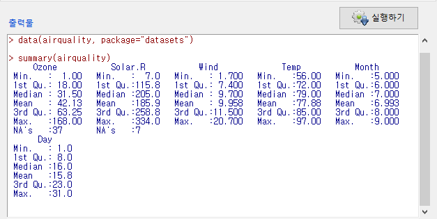
summary(faithful)
str(faithful)

Linux 사례 (MX 21)

데이터셋의 내부는 다음과 같다:

Linux 사례 (MX 21)

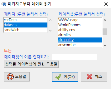
?faithful	# datasets 패키지에 포함된 faithful 데이터셋 도움말 보기


faithful {datasets} R Documentation

Old Faithful Geyser Data

Description

Waiting time between eruptions and the duration of the eruption for the Old Faithful geyser in Yellowstone National Park, Wyoming, USA.

Usage

faithful

Format

A data frame with 272 observations on 2 variables.

[,1] eruptions numeric Eruption time in mins
[,2] waiting numeric Waiting time to next eruption (in mins)
 

Details

A closer look at faithful$eruptions reveals that these are heavily rounded times originally in seconds, where multiples of 5 are more frequent than expected under non-human measurement. For a better version of the eruption times, see the example below.

There are many versions of this dataset around: Azzalini and Bowman (1990) use a more complete version.

Source

W. Härdle.

References

Härdle, W. (1991). Smoothing Techniques with Implementation in S. New York: Springer.

Azzalini, A. and Bowman, A. W. (1990). A look at some data on the Old Faithful geyser. Applied Statistics, 39, 357–365. doi: 10.2307/2347385.

See Also

geyser in package MASS for the Azzalini–Bowman version.

Examples

require(stats); require(graphics)
f.tit <-  "faithful data: Eruptions of Old Faithful"

ne60 <- round(e60 <- 60 * faithful$eruptions)
all.equal(e60, ne60)             # relative diff. ~ 1/10000
table(zapsmall(abs(e60 - ne60))) # 0, 0.02 or 0.04
faithful$better.eruptions <- ne60 / 60
te <- table(ne60)
te[te >= 4]                      # (too) many multiples of 5 !
plot(names(te), te, type = "h", main = f.tit, xlab = "Eruption time (sec)")

plot(faithful[, -3], main = f.tit,
     xlab = "Eruption time (min)",
     ylab = "Waiting time to next eruption (min)")
lines(lowess(faithful$eruptions, faithful$waiting, f = 2/3, iter = 3),
      col = "red")

[Package datasets version 4.0.4 Index]

'Dataset_info > faithful' 카테고리의 다른 글

faithful 데이터셋 예제  (0) 2022.07.25

carData::Duncan()

Linux 사례 (MX 21)
Linux 사례 (MX 21)

data(Duncan, package="carData")

R Commander의 상단에 있는 '데이터셋 보기' 버튼을 누르면, 아래와 같이 데이터셋 내부를 볼 수 있다.

Linux 사례 (MX 21)
Linux 사례 (MX 21)

?Duncan    # Duncan 데이터셋 도움말 보기

Duncan {carData} R Documentation

Duncan's Occupational Prestige Data

Description

The Duncan data frame has 45 rows and 4 columns. Data on the prestige and other characteristics of 45 U. S. occupations in 1950.

Usage

Duncan

Format

This data frame contains the following columns:

type

Type of occupation. A factor with the following levels: prof, professional and managerial; wc, white-collar; bc, blue-collar.

income

Percentage of occupational incumbents in the 1950 US Census who earned $3,500 or more per year (about $36,000 in 2017 US dollars).

education

Percentage of occupational incumbents in 1950 who were high school graduates (which, were we cynical, we would say is roughly equivalent to a PhD in 2017)

prestige

Percentage of respondents in a social survey who rated the occupation as “good” or better in prestige

Source

Duncan, O. D. (1961) A socioeconomic index for all occupations. In Reiss, A. J., Jr. (Ed.) Occupations and Social Status. Free Press [Table VI-1].

References

Fox, J. (2016) Applied Regression Analysis and Generalized Linear Models, Third Edition. Sage.

Fox, J. and Weisberg, S. (2019) An R Companion to Applied Regression, Third Edition, Sage.


[Package carData version 3.0-4 Index]

datasets::warpbreaks()

Linux 사례 (MX 21)

data(warpbreaks, package="datasets") # 데이터셋 불러오기	
help("warpbreaks")                   # 데이터셋 도움말 보기
summary(warpbreaks)                  # 데이터셋 통계 요약 보기

Linux 사례 (MX 21)

R Commander 화면 상단 우측에 있는 <데이터셋 보기> 버튼을 누른다. 아래와 같이 warpbreaks 데이터셋의 내부 구성을 볼 수 있다.

Linux 사례 (MX 21)


warpbreaks {datasets} R Documentation

The Number of Breaks in Yarn during Weaving

Description

This data set gives the number of warp breaks per loom, where a loom corresponds to a fixed length of yarn.

Usage

warpbreaks

Format

A data frame with 54 observations on 3 variables.

[,1] breaks numeric The number of breaks
[,2] wool factor The type of wool (A or B)
[,3] tension factor The level of tension (L, M, H)

There are measurements on 9 looms for each of the six types of warp (AL, AM, AH, BL, BM, BH).

Source

Tippett, L. H. C. (1950) Technological Applications of Statistics. Wiley. Page 106.

References

Tukey, J. W. (1977) Exploratory Data Analysis. Addison-Wesley.

McNeil, D. R. (1977) Interactive Data Analysis. Wiley.

See Also

xtabs for ways to display these data as a table.

Examples

require(stats); require(graphics)
summary(warpbreaks)
opar <- par(mfrow = c(1, 2), oma = c(0, 0, 1.1, 0))
plot(breaks ~ tension, data = warpbreaks, col = "lightgray",
     varwidth = TRUE, subset = wool == "A", main = "Wool A")
plot(breaks ~ tension, data = warpbreaks, col = "lightgray",
     varwidth = TRUE, subset = wool == "B", main = "Wool B")
mtext("warpbreaks data", side = 3, outer = TRUE)
par(opar)
summary(fm1 <- lm(breaks ~ wool*tension, data = warpbreaks))
anova(fm1)

[Package datasets version 4.0.4 Index]

'Dataset_info > warpbreaks' 카테고리의 다른 글

warpbreaks 데이터셋 예제  (0) 2022.06.25

carData::Adler

Linux 사례 (MX 21)

데이터 > 패키지에 있는 데이터 > 첨부된 패키지에서 데이터셋 읽기... 기능을 선택하면, 위와 같은 메뉴 창을 보게된다.

carData를 선택하여 두번 클릭하면, 오른쪽에 carData 패키지에 내장된 데이터셋 목록이 등장한다. Adler 데이터셋을 선택한다.

Linux 사례 (MX 21)

data(Adler, package="carData")  # Adler 데이터셋 활성화시키기
help("Adler", package="carData")# 도움말파일 열기

Linux사례 (MX 21)


Adler {carData} R Documentation

Experimenter Expectations

Description

The Adler data frame has 108 rows and 3 columns.

The “experimenters” were the actual subjects of the study. They collected ratings of the apparent success of people in pictures who were pre-selected for their average appearance of success. The experimenters were told prior to collecting data that particular subjects were either high or low in their tendency to rate appearance of success, and were instructed to get good data, scientific data, or were given no such instruction. Each experimenter collected ratings from 18 randomly assigned subjects. This version of the Adler data is taken from Erickson and Nosanchuk (1977). The data described in the original source, Adler (1973), have a more complex structure.

Usage

Adler

Format

This data frame contains the following columns:

instruction

a factor with levels: good, good data; none, no stress; scientific, scientific data.

expectation

a factor with levels: high, expect high ratings; low, expect low ratings.

rating

The average rating obtained.

Source

Erickson, B. H., and Nosanchuk, T. A. (1977) Understanding Data. McGraw-Hill Ryerson.

References

Adler, N. E. (1973) Impact of prior sets given experimenters and subjects on the experimenter expectancy effect. Sociometry 36, 113–126.

모델 > 모델 요약하기

Models > Summarize model

Linux 요약 (MX 21)

모델을 만들고, 모델의 요약 정보를 확인할 때 일반적으로 summary() 함수를 사용한다.

carData 패키지의 Prestige 데이터셋으로 선형회귀, 선형모델을 만들었다고 하자. 이 과정에서 다음 사례와 같은 요약 정보가 생산된다:

summary(LinearModel.2)

Linux 사례(MX 21)

여러개의 모델이 있고, 특정 모델의 요약정보를 다시 확인하고자 할 때 사용하는 기능이다.

Linux 사례 (MX 21)

<계수 표준 오차의 샌드위치 추정치 사용하기>에 선택이 되어 있는 경우는 summary() 함수 대신 summarySandwich() 함수가 사용된다.

Linux 사례 (MX 21)

summarySandwich(LinearModel.2, type="hc3")

Linux 사례 (MX 21)

datasets::airquality()

Linux 사례 (MX 21)

R이 시작될 때, datasets 패키지가 자동으로 호출된다. 따라서 R Commander를 실행할 때, datasets 패키지는 첨부 패키지화되어 메뉴창을 통해서 내부 데이터셋을 찾고 불러올 수 있다.

메뉴창에서 순서대로 데이터 > 패키지에 있는 데이터 > 첨부된 패키지에서 데이터셋 읽기... 를 선택하면 다음과 같은 창이 등장한다.

Windows 사례

출력창을 보면, airquality라는 데이터셋에는 6개의 변수가 있고, 각 변수는 수치형 정보를 담고 있다.

Windows 사례

Month 변수는 최소 5에서 최대 9로 값이 있는데, 정확히는 5월부터 9월까지일 것이다. 한달 한달을 뜻하는 월(month)은 5월이 9월보다 크다고 할 수 없고, 5월, 6월, 7월, 8월, 9월 등으로 개체화되어 분리된다. 다시 말하면, 요인형 변수가 되어야 한다는 뜻이다.

그럼 왜, airqualty 데이터셋의 Month 변수는 수치형으로 되어 있을까. 원자료를 R의 데이터셋으로 불러오는 과정에서 해당 변수의 요인화과정이 생략되었을 것이다.


airquality {datasets} R Documentation

New York Air Quality Measurements

Description

Daily air quality measurements in New York, May to September 1973.

Usage

airquality

Format

A data frame with 153 observations on 6 variables.

[,1] Ozone numeric Ozone (ppb)
[,2] Solar.R numeric Solar R (lang)
[,3] Wind numeric Wind (mph)
[,4] Temp numeric Temperature (degrees F)
[,5] Month numeric Month (1--12)
[,6] Day numeric Day of month (1--31)

Details

Daily readings of the following air quality values for May 1, 1973 (a Tuesday) to September 30, 1973.

  • Ozone: Mean ozone in parts per billion from 1300 to 1500 hours at Roosevelt Island
  • Solar.R: Solar radiation in Langleys in the frequency band 4000–7700 Angstroms from 0800 to 1200 hours at Central Park
  • Wind: Average wind speed in miles per hour at 0700 and 1000 hours at LaGuardia Airport
  • Temp: Maximum daily temperature in degrees Fahrenheit at La Guardia Airport.

Source

The data were obtained from the New York State Department of Conservation (ozone data) and the National Weather Service (meteorological data).

References

Chambers, J. M., Cleveland, W. S., Kleiner, B. and Tukey, P. A. (1983) Graphical Methods for Data Analysis. Belmont, CA: Wadsworth.

Examples

require(graphics)
pairs(airquality, panel = panel.smooth, main = "airquality data")

[Package datasets version 4.0.4 Index]

'Dataset_info > airquality' 카테고리의 다른 글

airquality 데이터셋 예제  (0) 2022.06.24

통계 > 요약 > 활성 데이터셋
Statistics > Summaries > Active Data set

Linux 사례 (Ubuntu 18.04)


Prestige라는 데이터셋을 불러와서 자료처리와 분석용으로 활성화시켰다고 가정하자. Prestige 데이터셋의 요약정보를 보고자 할때, <활성 데이터셋> 기능을 선택한다:

data(Prestige)
summary(Prestige)

Linux 사례 (Ubuntu 18.04)


?summary  # base 패키지의 summary 도움말 보기

summary(attenu, digits = 4) #-> summary.data.frame(...), default precision
summary(attenu $ station, maxsum = 20) #-> summary.factor(...)

lst <- unclass(attenu$station) > 20 # logical with NAs
## summary.default() for logicals -- different from *.factor:
summary(lst)
summary(as.factor(lst))

'Statistics > Summaries' 카테고리의 다른 글

6. Correlation matrix...  (0) 2022.02.13
5. Table of Statistics...  (0) 2022.02.13
4. Count missing observations  (0) 2022.02.13
3. Frequency distributions...  (0) 2022.02.13
2. Numeric summaries...  (0) 2022.02.13

데이터 > 활성 데이터셋의 변수 관리하기 > 수치 변수를 요인으로 변환하기...
Data > Manage variables in active data set > Convert numeric variable to factor...

Windows 사례


수치 변수를 요인으로 전환해야 하는 경우가 흔하다. 남성을 1, 여성을 2로 입력한 엑셀 자료를 불러오는 경우, 1과 2를 요인으로 재지정해야 남성, 여성의 의미를 담은 변수로 활용할 수 있다. 일반적으로 이런 변수를 명목변수(nominal variable)이라고 하지만, R에서는 factor (variable)로 부른다. 간혹 요인분석에 익숙한 사용자가 factor와 factor analysis를 헷갈려하는 경우가 있기도 하다.

수치 변수인가? 요인 인가? 변수의 유형에 대한 이해가 필요한 이유는 실용적으로 볼 때, 시각화와 연결된 작업때문이다. 줄여 말하면, 수치 변수로 표현할 수 있는 시각화와 요인으로 표현할 시각화 기법이 다르다고 할 수 있다. 어려운가? 간단히 예를 들면, 히스토그램은 수치 변수의 시각화 기법이다. 그러나, 막대 차트는 요인의 시각화 기법이다. 수치 변수는 더할 수 있고, 요인은 셀 수 있다.

먼저 datasets 패키지에 있는 airquality 데이터셋을 활성화시키자.

https://rcmdr.tistory.com/100


airquality 데이터셋 요약 정보

R이 시작될 때, datasets 패키지가 자동으로 호출된다. 따라서 R Commander를 실행할 때, datasets 패키지는 첨부 패키지화되어 메뉴창을 통해서 내부 데이터셋을 찾고 불러올 수 있다. 메뉴창에서 순서

rcmdr.kr


작업창에는 '다중 변수를 위한 새로운 변수 이름 또는 접미사: <변수와 똑같음>' 이라는 조건입력칸이 있다. 변수 이름을 덮어쓰면서, 바뀐 변수 유형을 기억하기도 하지만, 나는 흔히 _f를 추가한다. 원래의 수치 변수 옆에 _f가 붙어있는 요인을 만들어 그 차이를 기억하는 방식이다.

Linux 사례 (MX 21)

데이터셋 <- with(데이터셋, {요인형변수이름 <- as.factor(수치형변수) })

airquality <- within(airquality, { month.f <- as.factor(Month) })


참고로, 간혹 다음의 오류 지시문 "수준의 숫자 ( ) (이)가 너무 넓습니다"이 아래 알림글에 나올 수 있다. 이것은 요인화로 만들어지는 수준의 갯수가 너무 많다는 의미이다. 그래서 요인 수준 이름을 일일이 넣을 추가 작업창을 R Commander에서 만들 수 없다는 뜻이다. 작업창의 요인 수준에서 "수준 이름 사용하기"를 선택 (기본선택사항)해서 이와 같은 오류 지시문이 나오는 경우, 그 아래에 있는 "숫자 사용하기" 선택을 하면 된다.

아래 출력창에서 airquality 데이터셋의 Month 변수와 month.f 변수를 비교해보자. Month 변수는 수치형 변수로서 최소, 평균, 최대 값을 갖고 있는 반면에, month.f 변수는 5에 31, 7에 31, 9에 30 등의 갯수를 갖고 있다.

Linux 사례 (MX 21)


?factor  # base 패키지의 factor 도움말 보기

(ff <- factor(substring("statistics", 1:10, 1:10), levels = letters))
as.integer(ff)      # the internal codes
(f. <- factor(ff))  # drops the levels that do not occur
ff[, drop = TRUE]   # the same, more transparently

factor(letters[1:20], labels = "letter")

class(ordered(4:1)) # "ordered", inheriting from "factor"
z <- factor(LETTERS[3:1], ordered = TRUE)
## and "relational" methods work:
stopifnot(sort(z)[c(1,3)] == range(z), min(z) < max(z))


## suppose you want "NA" as a level, and to allow missing values.
(x <- factor(c(1, 2, NA), exclude = NULL))
is.na(x)[2] <- TRUE
x  # [1] 1    <NA> <NA>
is.na(x)
# [1] FALSE  TRUE FALSE

## More rational, since R 3.4.0 :
factor(c(1:2, NA), exclude =  "" ) # keeps <NA> , as
factor(c(1:2, NA), exclude = NULL) # always did
## exclude = <character>
z # ordered levels 'A < B < C'
factor(z, exclude = "C") # does exclude
factor(z, exclude = "B") # ditto

## Now, labels maybe duplicated:
## factor() with duplicated labels allowing to "merge levels"
x <- c("Man", "Male", "Man", "Lady", "Female")
## Map from 4 different values to only two levels:
(xf <- factor(x, levels = c("Male", "Man" , "Lady",   "Female"),
                 labels = c("Male", "Male", "Female", "Female")))
#> [1] Male   Male   Male   Female Female
#> Levels: Male Female

## Using addNA()
Month <- airquality$Month
table(addNA(Month))
table(addNA(Month, ifany = TRUE))

'Data > Manage variables in active data set' 카테고리의 다른 글

11. Rename variables...  (0) 2020.03.21
7. Bin a numeric variable...  (0) 2020.03.21
4. Standardize variables...  (0) 2019.09.08
3. Add observation number to data set  (0) 2019.09.08
2. Compute new variable...  (0) 2019.09.08

+ Recent posts