통계 > 요약 > 정규성을 향해서 변환시키기...

Statistics > Summaries > Transform toward normaltiy...


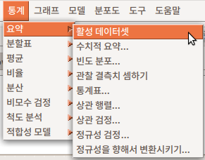
어느 데이터셋을 활성화시키면, '통계 > 요약 > 정규성을 향해서 변환시키기...' 메뉴 기능이 아래와 같이 활성화될 것이다.

Linux 사례 (MX 21)

carData 패키지에 포함된 Prestige 데이터셋을 이용하여 연습해보자.

'데이터 > 패키지에 있는 데이터 > 첨부된 패키지에서 데이터셋 읽기...' 메뉴 기능을 선택한후 carData 패키지에 있는 Prestige 데이터셋을 찾아서 선택한다. 그러면, R Commander 상단에 있는 <활성 데이터셋 없음> 이라는 버튼이 'Prestige'로 바뀌면서 '통계 > 요약 > 정규성을 향해서 변환하기...' 메뉴 기능을 이용할 수 있게 된다. 이 메뉴를 선택한다. 그러면, 아래와 같은 화면이 등장한다.  Prestige 데이터셋에서 정규성을 향해서 변환시킬 변수를 선택하는 메뉴 창인데, income 변수를 선택해보자.

Linux 사례 (MX 21)

car 패키지에 포함된 powerTransform() 함수를 사용하여 출력창에 아래와 같은 결과를 생산한다. 출력내용에서 'Est Power'값으로 제시하는 0.1793을 확인한다. Prestige 패키지에 있는 income 변수에 0.1793 승(제곱)을 하면, 그 사례 값들은 정규 분포적 특성으로 변환될 수 있다는 의미이다.

Linux 사례 (MX 21)


'통계 > 요약 > 정규성 검정...' 메뉴 기능이 있다. 이 기능을 사용하여, Prestige 데이터셋의 income 변수와 정규성을 향해서 변환된 income 변수의 새로운 변수, 편의상 variable_Income,의 정규성 검정을 시도해보자.

https://rcmdr.kr/88


8. Test of normality...

통계 > 요약 > 정규성 검정... Statistics > Summaries > Test of normality... 수치형(numeric, integer) 변수들 중에서 하나를 선택한다. 기본 설정에 Shapiro-Wilk의 정규성 검정법이 선택되어 있다. 수입(연..

rcmdr.kr

먼저, 변환된 변수를 Prestige 데이터셋에 추가해야 한다. '데이터 > 활성 데이터셋에 있는 변수 관리하기 > 새로운 변수 계산하기...' 메뉴 기능을 통하여 income 변수가 변환된 variable_Income 변수를 만들어보자. '계산 표현식'에 income^0.1793이 입력된 것을 확인한다. 여기서 0.1793은 powerTransform() 함수를 통하여 앞서 추출한 income 변수의 승(제곱) 값이다.

Linux 사례 (MX 21)

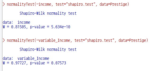
Prestige 데이터셋에 variable_Income 이라는 새로운 변수가 추가된다. 이제 '통계 > 요약 > 정규성 검정...' 메뉴 기능을 선택하고, 차례로 두번의 정규성 검정을 진행한다. 첫번째는 income 변수로, 두번째는 variable_Income변수를 선택한다. 두개의 정규성 검정 결과를 비교하기 위해서다. 아래 화면은 두번째 검정, variable_Income 변수를 선택하는 메뉴 창이다.

Linux 사례 (MX 21)

두번의 정규성 검정에서 제시하는 유의 확률값을 살펴보자. variable_Income 변수의 정규성 검정 결과는 p-value=0.07573으로 variable _income 변수는 정규분포적 특징을 갖는다고 할 수 있다.

Linux 사례 (MX 21)


?powerTransform  # car 패키지의 powerTransform 도움말 보기

# Box Cox Method, univariate
summary(p1 <- powerTransform(cycles ~ len + amp + load, Wool))
# fit linear model with transformed response:
coef(p1, round=TRUE)
summary(m1 <- lm(bcPower(cycles, p1$roundlam) ~ len + amp + load, Wool))

# Multivariate Box Cox uses Highway1 data
summary(powerTransform(cbind(len, adt, trks, sigs1) ~ 1, Highway1))

# Multivariate transformation to normality within levels of 'htype'
summary(a3 <- powerTransform(cbind(len, adt, trks, sigs1) ~ htype, Highway1))

# test lambda = (0 0 0 -1)
testTransform(a3, c(0, 0, 0, -1))

# save the rounded transformed values, plot them with a separate
# color for each highway type
transformedY <- bcPower(with(Highway1, cbind(len, adt, trks, sigs1)),
                        coef(a3, round=TRUE))
## Not run: scatterplotMatrix( ~ transformedY|htype, Highway1) 

# With negative responses, use the bcnPower family
m2 <- lm(I1L1 ~ pool, LoBD)
summary(p2 <- powerTransform(m2, family="bcnPower"))
testTransform(p2, .5)
summary(powerTransform(update(m2, cbind(LoBD$I1L2, LoBD$I1L1) ~ .), family="bcnPower"))

## Not run:  
  # takes a few seconds:
  # multivariate bcnPower, with 8 responses
  summary(powerTransform(update(m2, as.matrix(LoBD[, -1]) ~ .), family="bcnPower"))
  # multivariate bcnPower, fit with one iteration using starting values as estimates
  summary(powerTransform(update(m2, as.matrix(LoBD[, -1]) ~ .), family="bcnPower", itmax=1))

## End(Not run)

# mixed effects model
## Not run: 
  # uses the lme4 package
  data <- reshape(LoBD[1:20, ], varying=names(LoBD)[-1], direction="long", v.names="y")
  names(data) <- c("pool", "assay", "y", "id")
  data$assay <- factor(data$assay)
  require(lme4)
  m2 <- lmer(y ~ pool + (1|assay), data)
  summary(l2 <- powerTransform(m2, family="bcnPower", verbose=TRUE))

## End(Not run)

'Statistics > Summaries' 카테고리의 다른 글

8. Test of normality...  (0) 2022.02.13
7. Correlation test...  (0) 2022.02.13
6. Correlation matrix...  (0) 2022.02.13
5. Table of Statistics...  (0) 2022.02.13
4. Count missing observations  (0) 2022.02.13

통계 > 요약 > 정규성 검정...

Statistics > Summaries > Test of normality...


Linux 사례 (Ubuntu 18.04)

수치형(numeric, integer) 변수들 중에서 하나를 선택한다. 기본 설정에 Shapiro-Wilk의 정규성 검정법이 선택되어 있다. 수입(연봉)의 사례들이 정규 분포를 이루고 있는가를 확인하고자, 변수 income을 선택하고 예(OK) 버튼을 누른다.

Linux 사례 (Ubuntu 18.04)

normalityTest()를 사용한다.

Linux 사례 (Ubuntu 18.04)


normalityTest(~education, test="shapiro.test", data=Prestige)

Linux 사례 (MX 21)


?normalityTest  # RcmdrMisc 패키지의 normalityTest 도움말 보기

data(Prestige, package="car")
  with(Prestige, normalityTest(income))
  normalityTest(income ~ type, data=Prestige, test="ad.test")
  normalityTest(~income, data=Prestige, test="pearson.test", n.classes=5)

'Statistics > Summaries' 카테고리의 다른 글

9. Transform toward normality...  (0) 2022.06.19
7. Correlation test...  (0) 2022.02.13
6. Correlation matrix...  (0) 2022.02.13
5. Table of Statistics...  (0) 2022.02.13
4. Count missing observations  (0) 2022.02.13

통계 > 요약 > 상관 검정...
Statistics > Summaries > Correlation test...

Linux 사례 (Ubuntu 18.04)

상관 검정은 두 변수를 구성하는 사례값들 사이에 어떤 방향의 관계성이 있는지를 통계학적으로 확인하고자 할 때 사용한다. 아래는Prestige 데이터셋에서 교육수준과 수입(연봉) 사이에 어떤 관계성이 있는지를 확인하고자 한다. education과 income 변수를 선택하고, 예(OK) 버튼을 누른다.

Linux 사례 (Ubuntu 18.04)

상관의 유형 중에서 Pearson product-moment (피어슨 적률상관), 대립 가설에는 양측이 기본으로 설정되어 있다. 이 설정을 바탕으로 상관 검증의 결과를 출력하면 아래와 같다:

Linux 사례 (Ubuntu 18.04)

cor.test() 함수를 활용한다.


?cor.test  # stats 패키지의 cor.test 도움말 보기

## Hollander & Wolfe (1973), p. 187f.
## Assessment of tuna quality.  We compare the Hunter L measure of
##  lightness to the averages of consumer panel scores (recoded as
##  integer values from 1 to 6 and averaged over 80 such values) in
##  9 lots of canned tuna.

x <- c(44.4, 45.9, 41.9, 53.3, 44.7, 44.1, 50.7, 45.2, 60.1)
y <- c( 2.6,  3.1,  2.5,  5.0,  3.6,  4.0,  5.2,  2.8,  3.8)

##  The alternative hypothesis of interest is that the
##  Hunter L value is positively associated with the panel score.

cor.test(x, y, method = "kendall", alternative = "greater")
## => p=0.05972

cor.test(x, y, method = "kendall", alternative = "greater",
         exact = FALSE) # using large sample approximation
## => p=0.04765

## Compare this to
cor.test(x, y, method = "spearm", alternative = "g")
cor.test(x, y,                    alternative = "g")

## Formula interface.
require(graphics)
pairs(USJudgeRatings)
cor.test(~ CONT + INTG, data = USJudgeRatings)

'Statistics > Summaries' 카테고리의 다른 글

9. Transform toward normality...  (0) 2022.06.19
8. Test of normality...  (0) 2022.02.13
6. Correlation matrix...  (0) 2022.02.13
5. Table of Statistics...  (0) 2022.02.13
4. Count missing observations  (0) 2022.02.13

통계 > 요약 > 상관 행렬...
Statistics > Summaries > Correlation matrix...

Linux 사례 (Ubuntu 18.04)

상관 행렬은 두개 이상의 변수를 선택해야 한다. Prestige 데이터셋에서 교육수준과 연봉(수입)의 관계에 대한 관심에서 이 두 변수를 선택하고, 예(OK) 버튼을 누른다.

Linux 사례 (Ubuntu 18.04)


Linux 사례 (Ubuntu 18.04)

출력 창을 보면, cor() 함수가 사용되었음을 알 수 있다.


?rcorr.adjust  #RcmdrMisc 패키지의 rcorr.adjust 도움말 보기

if (require(car)){
    data(Mroz)
    print(rcorr.adjust(Mroz[,c("k5", "k618", "age", "lwg", "inc")]))
    print(rcorr.adjust(Mroz[,c("k5", "k618", "age", "lwg", "inc")], type="spearman"))
    }

'Statistics > Summaries' 카테고리의 다른 글

8. Test of normality...  (0) 2022.02.13
7. Correlation test...  (0) 2022.02.13
5. Table of Statistics...  (0) 2022.02.13
4. Count missing observations  (0) 2022.02.13
3. Frequency distributions...  (0) 2022.02.13

통계 > 요약 > 통계표...
Statistics > Summaries > Table of statistics...

Linux 사례 (Ubuntu 18.04)

통계표(Table of statistics)는 요인(factor) 변수 유형별로 수치형(numeric, integer) 변수의 통계량을 계산하여 출력한다. Prestige 데이터셋에서 직업 유형의 type 변수를 요인에서 선택하고, 직업 유형별로 권위(prestige)의 통계량 중에서 기본 설정으로 선택된 평균값의 통계표를 선택하고, 예(OK) 버튼을 누른다.

Linux 사례 (Ubuntu 18.04)

직업 유형(bc, prof, wc)별로 평균값을 계산하여 출력한다. 출력창을 보면 Tapply() 함수를 사용함을 알 수 있다.


?Tapply  # car 패키지의 Tapply 도움말 보기

Tapply(conformity ~ partner.status + fcategory, mean, data=Moore)
Tapply(conformity ~ partner.status + fcategory, mean, data=Moore, 
    trim=0.2)

Moore[1, 2] <- NA
Tapply(conformity ~ partner.status + fcategory, mean, data=Moore)
Tapply(conformity ~ partner.status + fcategory, mean, data=Moore, 
  na.rm=TRUE)
Tapply(conformity ~ partner.status + fcategory, mean, data=Moore, 
  na.action=na.omit)  # equivalent
remove("Moore")

'Statistics > Summaries' 카테고리의 다른 글

7. Correlation test...  (0) 2022.02.13
6. Correlation matrix...  (0) 2022.02.13
4. Count missing observations  (0) 2022.02.13
3. Frequency distributions...  (0) 2022.02.13
2. Numeric summaries...  (0) 2022.02.13

통계 > 요약 > 관측 결측치 셈하기
Statistics > Summaries > Count missing observations

Linux 사례 (Ubuntu 18.04)

데이터셋을 구성하는 사례에 값이 입력되지 않은 결측치가 있는 경우가 있다. 어떤 변수에 관측값이 없는 결측치가 있는지를 확인할 때 사용하는 기능이다.

Linux 사례 (Ubuntu 18.04)


Prestige 데이터셋의 type 변수에 결측치가 4개가 있음을 확인한다.


?sapply  # base 패키지의  sapply 도움말 보기

require(stats); require(graphics)

x <- list(a = 1:10, beta = exp(-3:3), logic = c(TRUE,FALSE,FALSE,TRUE))
# compute the list mean for each list element
lapply(x, mean)
# median and quartiles for each list element
lapply(x, quantile, probs = 1:3/4)
sapply(x, quantile)
i39 <- sapply(3:9, seq) # list of vectors
sapply(i39, fivenum)
vapply(i39, fivenum,
       c(Min. = 0, "1st Qu." = 0, Median = 0, "3rd Qu." = 0, Max. = 0))

## sapply(*, "array") -- artificial example
(v <- structure(10*(5:8), names = LETTERS[1:4]))
f2 <- function(x, y) outer(rep(x, length.out = 3), y)
(a2 <- sapply(v, f2, y = 2*(1:5), simplify = "array"))
a.2 <- vapply(v, f2, outer(1:3, 1:5), y = 2*(1:5))
stopifnot(dim(a2) == c(3,5,4), all.equal(a2, a.2),
          identical(dimnames(a2), list(NULL,NULL,LETTERS[1:4])))

hist(replicate(100, mean(rexp(10))))

## use of replicate() with parameters:
foo <- function(x = 1, y = 2) c(x, y)
# does not work: bar <- function(n, ...) replicate(n, foo(...))
bar <- function(n, x) replicate(n, foo(x = x))
bar(5, x = 3)

'Statistics > Summaries' 카테고리의 다른 글

6. Correlation matrix...  (0) 2022.02.13
5. Table of Statistics...  (0) 2022.02.13
3. Frequency distributions...  (0) 2022.02.13
2. Numeric summaries...  (0) 2022.02.13
1. Active Data set  (0) 2022.02.13

통계 > 요약 > 빈도 분포...
Statistics > Summaries > Frequency distributions...

Linux 사례 (Ubuntu 18.04)


type 변수를 선택하고 예(OK)를 누른다. Prestige 데이터셋의 type 변수의 빈도를 보는 명령문이 다음과 같이 입력창에 기록되고 출력창에 빈도 정보가 출력된다:

Linux 사례 (Ubuntu 18.04) - 입력 창 기록
Linux 사례 (Ubuntu 18.04) - 출력창 출력결과


더보기

Q1> Prestige의 변수는 여러개가 있습니다. 그중에서 왜 type만 선택 창에 나오나요?


type 변수는 factor 유형입니다. 빈도는 factor 유형의 변수만 셀 수 있기 때문입니다.

> str(Prestige) # Prestige 데이터셋의 변수 유형 살펴보기


?table  # base 패키지의 table 도움말 보기

require(stats) # for rpois and xtabs
## Simple frequency distribution
table(rpois(100, 5))
## Check the design:
with(warpbreaks, table(wool, tension))
table(state.division, state.region)

# simple two-way contingency table
with(airquality, table(cut(Temp, quantile(Temp)), Month))

a <- letters[1:3]
table(a, sample(a))                    # dnn is c("a", "")
table(a, sample(a), deparse.level = 0) # dnn is c("", "")
table(a, sample(a), deparse.level = 2) # dnn is c("a", "sample(a)")

## xtabs() <-> as.data.frame.table() :
UCBAdmissions ## already a contingency table
DF <- as.data.frame(UCBAdmissions)
class(tab <- xtabs(Freq ~ ., DF)) # xtabs & table
## tab *is* "the same" as the original table:
all(tab == UCBAdmissions)
all.equal(dimnames(tab), dimnames(UCBAdmissions))

a <- rep(c(NA, 1/0:3), 10)
table(a)                 # does not report NA's
table(a, exclude = NULL) # reports NA's
b <- factor(rep(c("A","B","C"), 10))
table(b)
table(b, exclude = "B")
d <- factor(rep(c("A","B","C"), 10), levels = c("A","B","C","D","E"))
table(d, exclude = "B")
print(table(b, d), zero.print = ".")

## NA counting:
is.na(d) <- 3:4
d. <- addNA(d)
d.[1:7]
table(d.) # ", exclude = NULL" is not needed
## i.e., if you want to count the NA's of 'd', use
table(d, useNA = "ifany")

## "pathological" case:
d.patho <- addNA(c(1,NA,1:2,1:3))[-7]; is.na(d.patho) <- 3:4
d.patho
## just 3 consecutive NA's ? --- well, have *two* kinds of NAs here :
as.integer(d.patho) # 1 4 NA NA 1 2
##
## In R >= 3.4.0, table() allows to differentiate:
table(d.patho)                   # counts the "unusual" NA
table(d.patho, useNA = "ifany")  # counts all three
table(d.patho, exclude = NULL)   #  (ditto)
table(d.patho, exclude = NA)     # counts none

## Two-way tables with NA counts. The 3rd variant is absurd, but shows
## something that cannot be done using exclude or useNA.
with(airquality,
   table(OzHi = Ozone > 80, Month, useNA = "ifany"))
with(airquality,
   table(OzHi = Ozone > 80, Month, useNA = "always"))
with(airquality,
   table(OzHi = Ozone > 80, addNA(Month)))

'Statistics > Summaries' 카테고리의 다른 글

6. Correlation matrix...  (0) 2022.02.13
5. Table of Statistics...  (0) 2022.02.13
4. Count missing observations  (0) 2022.02.13
2. Numeric summaries...  (0) 2022.02.13
1. Active Data set  (0) 2022.02.13

통계 > 요약 > 수치적 요약...
Statistics > Summaries > Numeric summaries...

Linux 사례 (Ubuntu 18.04)


<수치적 요약...> 메뉴를 선택하면 하위 창이 나온다:

Linux 사례 (Ubunt 18.04)


데이터 창과 통계 창이 있다. 통계 창을 보려면 데이터 옆에 있는 통계 창을 선택하면 된다:

Linux 사례 (Ubuntu 18.04)


다시 데이터 창으로 와서 prestige 라는 변수의 수치적 요약 정보를 보고자 한다. prestige 변수를 선택하고, 오른쪽 아래의 예(OK) 버튼을 선택한다:

Linux 사례 (Ubuntu 18.04)


입력 창과 출력 창을 살펴보자. 통계 창의 선택사항들에 변경을 주지 않은 상태에서 Prestige 라는 데이터셋의 prestige 변수의 수치적 정보는 다음과 같다:

Linux 사례 (Ubuntu 18.04)


?numSummary  # RcmdrMisc 패키지의 numSummary 도움말 보기

if (require("car")){
    data(Prestige)
    Prestige[1, "income"] <- NA
    print(numSummary(Prestige[,c("income", "education")], 
    	statistics=c("mean", "sd", "quantiles", "cv", "skewness", "kurtosis")))
    print(numSummary(Prestige[,c("income", "education")], groups=Prestige$type))
    remove(Prestige)
}

'Statistics > Summaries' 카테고리의 다른 글

6. Correlation matrix...  (0) 2022.02.13
5. Table of Statistics...  (0) 2022.02.13
4. Count missing observations  (0) 2022.02.13
3. Frequency distributions...  (0) 2022.02.13
1. Active Data set  (0) 2022.02.13

통계 > 요약 > 활성 데이터셋
Statistics > Summaries > Active Data set

Linux 사례 (Ubuntu 18.04)


Prestige라는 데이터셋을 불러와서 자료처리와 분석용으로 활성화시켰다고 가정하자. Prestige 데이터셋의 요약정보를 보고자 할때, <활성 데이터셋> 기능을 선택한다:

data(Prestige)
summary(Prestige)

Linux 사례 (Ubuntu 18.04)


?summary  # base 패키지의 summary 도움말 보기

summary(attenu, digits = 4) #-> summary.data.frame(...), default precision
summary(attenu $ station, maxsum = 20) #-> summary.factor(...)

lst <- unclass(attenu$station) > 20 # logical with NAs
## summary.default() for logicals -- different from *.factor:
summary(lst)
summary(as.factor(lst))

'Statistics > Summaries' 카테고리의 다른 글

6. Correlation matrix...  (0) 2022.02.13
5. Table of Statistics...  (0) 2022.02.13
4. Count missing observations  (0) 2022.02.13
3. Frequency distributions...  (0) 2022.02.13
2. Numeric summaries...  (0) 2022.02.13

+ Recent posts