통계 > 분할표 > 다원표...

Statistics > Contingency tables >  Multi-way tables...

Linux 사례 (MX 21)

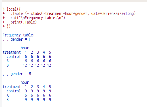
3개 이상의 요인형 변수를 포함하는 데이터셋이 활성화되면, '통계 > 분할표 > 다원표...' 메뉴 기능을 이용할 수 있다. 아래 메뉴 창에서 '통제 변수 (하나 이상 선택)'을 점검할 필요가 있다. 이원표를 만드는 기준 범주가 된다.

Linux 사례 (MX 21)
Linux 사례 (MX 21)


?xtabs  # stats 패키지의 xtabs 도움말 보기

## 'esoph' has the frequencies of cases and controls for all levels of
## the variables 'agegp', 'alcgp', and 'tobgp'.
xtabs(cbind(ncases, ncontrols) ~ ., data = esoph)
## Output is not really helpful ... flat tables are better:
ftable(xtabs(cbind(ncases, ncontrols) ~ ., data = esoph))
## In particular if we have fewer factors ...
ftable(xtabs(cbind(ncases, ncontrols) ~ agegp, data = esoph))

## This is already a contingency table in array form.
DF <- as.data.frame(UCBAdmissions)
## Now 'DF' is a data frame with a grid of the factors and the counts
## in variable 'Freq'.
DF
## Nice for taking margins ...
xtabs(Freq ~ Gender + Admit, DF)
## And for testing independence ...
summary(xtabs(Freq ~ ., DF))

## with NA's
DN <- DF; DN[cbind(6:9, c(1:2,4,1))] <- NA
DN # 'Freq' is missing only for (Rejected, Female, B)
tools::assertError(# 'na.fail' should fail :
     xtabs(Freq ~ Gender + Admit, DN, na.action=na.fail), verbose=TRUE)
op <- options(na.action = "na.omit") # the "factory" default
(xtabs(Freq ~ Gender + Admit, DN) -> xtD)
noC <- function(O) `attr<-`(O, "call", NULL)
ident_noC <- function(x,y) identical(noC(x), noC(y))
stopifnot(exprs = {
  ident_noC(xtD, xtabs(Freq ~ Gender + Admit, DN, na.action = na.omit))
  ident_noC(xtD, xtabs(Freq ~ Gender + Admit, DN, na.action = NULL))
})

xtabs(Freq ~ Gender + Admit, DN, na.action = na.pass)
## The Female:Rejected combination has NA 'Freq' (and NA prints 'invisibly' as "")
(xtNA <- xtabs(Freq ~ Gender + Admit, DN, addNA = TRUE)) # ==> count NAs
## show NA's better via  na.print = ".." :
print(xtNA, na.print= "NA")


## Create a nice display for the warp break data.
warpbreaks$replicate <- rep_len(1:9, 54)
ftable(xtabs(breaks ~ wool + tension + replicate, data = warpbreaks))

### ---- Sparse Examples ----

if(require("Matrix")) withAutoprint({
 ## similar to "nlme"s  'ergoStool' :
 d.ergo <- data.frame(Type = paste0("T", rep(1:4, 9*4)),
                      Subj = gl(9, 4, 36*4))
 xtabs(~ Type + Subj, data = d.ergo) # 4 replicates each
 set.seed(15) # a subset of cases:
 xtabs(~ Type + Subj, data = d.ergo[sample(36, 10), ], sparse = TRUE)

 ## Hypothetical two-level setup:
 inner <- factor(sample(letters[1:25], 100, replace = TRUE))
 inout <- factor(sample(LETTERS[1:5], 25, replace = TRUE))
 fr <- data.frame(inner = inner, outer = inout[as.integer(inner)])
 xtabs(~ inner + outer, fr, sparse = TRUE)
})

'Statistics > Contigency tables' 카테고리의 다른 글

3. Enter and analyze two-way table...  (0) 2022.06.28
Contingency tables  (0) 2022.02.14
1. Two-way table...  (0) 2022.02.14

통계 > 분할표 > 이원표 입력 및 분석하기...

Statistics > Contingency tables > Enter and analyze two-way table...

Linux 사례 (MX 21)

'통계 > 분할표 > 이원표 입력 및 분석하기...' 메뉴 기능을 선택하면 하위 창이 등장한다. '변수 이름', '행과 열의 수', '사례 수' 등을 입력할 수 있다. 아래의 내용은 'chisq.test' 함수 도움말 문서에 나오는 사례를 입력한다. 아래의 입력 스크립트를 참조 할 수 있다.

Linux 사례 (MX 21)
Linux 사례(MX 21)

.Table <- matrix(c(762,327,468,484,239,477), 2, 3, byrow=TRUE)
dimnames(.Table) <- list("Gender"=c("Female", "Male"), "Party"=c("Democrats", "Independent", 
  "Republican"))
.Table  # Counts
.Test <- chisq.test(.Table, correct=FALSE)
.Test
.Test$expected # Expected Counts

Linux 사례 (MX 21)


?chisq.test  # stats 패키지의  chisq.test 도움말 보기

## From Agresti(2007) p.39
M <- as.table(rbind(c(762, 327, 468), c(484, 239, 477)))
dimnames(M) <- list(gender = c("F", "M"),
                    party = c("Democrat","Independent", "Republican"))
(Xsq <- chisq.test(M))  # Prints test summary
Xsq$observed   # observed counts (same as M)
Xsq$expected   # expected counts under the null
Xsq$residuals  # Pearson residuals
Xsq$stdres     # standardized residuals


## Effect of simulating p-values
x <- matrix(c(12, 5, 7, 7), ncol = 2)
chisq.test(x)$p.value           # 0.4233
chisq.test(x, simulate.p.value = TRUE, B = 10000)$p.value
                                # around 0.29!

## Testing for population probabilities
## Case A. Tabulated data
x <- c(A = 20, B = 15, C = 25)
chisq.test(x)
chisq.test(as.table(x))             # the same
x <- c(89,37,30,28,2)
p <- c(40,20,20,15,5)
try(
chisq.test(x, p = p)                # gives an error
)
chisq.test(x, p = p, rescale.p = TRUE)
                                # works
p <- c(0.40,0.20,0.20,0.19,0.01)
                                # Expected count in category 5
                                # is 1.86 < 5 ==> chi square approx.
chisq.test(x, p = p)            #               maybe doubtful, but is ok!
chisq.test(x, p = p, simulate.p.value = TRUE)

## Case B. Raw data
x <- trunc(5 * runif(100))
chisq.test(table(x))            # NOT 'chisq.test(x)'!

'Statistics > Contigency tables' 카테고리의 다른 글

2. Multi-way tables...  (0) 2022.06.28
Contingency tables  (0) 2022.02.14
1. Two-way table...  (0) 2022.02.14

통계 > 분할표
Statistics > Contingency tables

Linux 사례 (MX 21)

분석대상인 데이터셋에 요인형 변수가 한개 있거나, 하나도 없는 경우 분할표 메뉴의 오른쪽에 있는 <이원표>, <다원표> 기능은 불활성 음영 표시로 나타난다. 두개 이상의 요인형 변수가 있는 경우, 예를 들어 car 패키지에 포함된 Moore 데이터셋이 활성 데이터셋이 되는 경우 불활성 음영 표시가 사라진다.

Linux 사례 (MX21)

요인형 변수가 세개 이상 있는 경우, <다원표> 까지 활성화된다. 아래의 화면을 보면, partner.status, fcatetory 두개의 변수가 요인(factor)형이다. <이원표>는 활성화된 반면에, <다원표> 기능이 아직 활성화되지 않았다면, 요인형 변수가 두개 뿐인 데이터셋임을 간접적으로 알려준다.

Linux 사례 (MX21)

'Statistics > Contigency tables' 카테고리의 다른 글

2. Multi-way tables...  (0) 2022.06.28
3. Enter and analyze two-way table...  (0) 2022.06.28
1. Two-way table...  (0) 2022.02.14

통계 > 분할표 > 이원표...
Statistics > Contingency tables > Two-way table...

Linux 사례 (MX 21)

요인형 변수를 두개 이상 가지고 있는 데이터셋이 활성화되었다면, '통계 > 분할표 > 이원표...' 메뉴 기능을 이용할 수 있다.

Linux 사례 (MX 21)


두개 이상의 요인형 변수를 가지고 있는 Moore 데이터셋을 활성화시키면, <이원표>의 음영이 사라지고 사용할 수 있는 기능이 된다.

Linux 사례 (MX 21)

행 변수와 열 변수에 요인형 변수 하나씩을 선택한다.

Linux 사례 (MX 21)
Linux 사례 (MX 21)

데이터 창과 함께 통계 창이 있다. 통계 창을 선택하면 다음과 같은 화면에 다양한 선택 기능을 선택할 수 있다. 다른 선택으로 출력 내용의 변화를 주지 않을 경우, 데이터 창으로 돌아가서 예(OK) 버튼을 누른다.

Linux 사례 (MX 21)

다음과 같은 출력물을 볼 수 있다. 행 변수에 partner.status, 열 변수에 fcategory를 선택한 경우의 출력물이다.

Linux 사례 (MX 21)

행 변수에 fcategory, 열 변수에 partner.status를 선택한 경우의 출력물이다.

Linux 사례 (MX 21)

프롬프트의 입력 스크립트를 살펴보면, xtabs() 함수를 사용하는 것이 보인다.


?xtabs  # stats 패키지의 xtabs 도움말 보기

## 'esoph' has the frequencies of cases and controls for all levels of
## the variables 'agegp', 'alcgp', and 'tobgp'.
xtabs(cbind(ncases, ncontrols) ~ ., data = esoph)
## Output is not really helpful ... flat tables are better:
ftable(xtabs(cbind(ncases, ncontrols) ~ ., data = esoph))
## In particular if we have fewer factors ...
ftable(xtabs(cbind(ncases, ncontrols) ~ agegp, data = esoph))

## This is already a contingency table in array form.
DF <- as.data.frame(UCBAdmissions)
## Now 'DF' is a data frame with a grid of the factors and the counts
## in variable 'Freq'.
DF
## Nice for taking margins ...
xtabs(Freq ~ Gender + Admit, DF)
## And for testing independence ...
summary(xtabs(Freq ~ ., DF))

## with NA's
DN <- DF; DN[cbind(6:9, c(1:2,4,1))] <- NA
DN # 'Freq' is missing only for (Rejected, Female, B)
tools::assertError(# 'na.fail' should fail :
     xtabs(Freq ~ Gender + Admit, DN, na.action=na.fail), verbose=TRUE)
op <- options(na.action = "na.omit") # the "factory" default
(xtabs(Freq ~ Gender + Admit, DN) -> xtD)
noC <- function(O) `attr<-`(O, "call", NULL)
ident_noC <- function(x,y) identical(noC(x), noC(y))
stopifnot(exprs = {
  ident_noC(xtD, xtabs(Freq ~ Gender + Admit, DN, na.action = na.omit))
  ident_noC(xtD, xtabs(Freq ~ Gender + Admit, DN, na.action = NULL))
})

xtabs(Freq ~ Gender + Admit, DN, na.action = na.pass)
## The Female:Rejected combination has NA 'Freq' (and NA prints 'invisibly' as "")
(xtNA <- xtabs(Freq ~ Gender + Admit, DN, addNA = TRUE)) # ==> count NAs
## show NA's better via  na.print = ".." :
print(xtNA, na.print= "NA")


## Create a nice display for the warp break data.
warpbreaks$replicate <- rep_len(1:9, 54)
ftable(xtabs(breaks ~ wool + tension + replicate, data = warpbreaks))

### ---- Sparse Examples ----

if(require("Matrix")) withAutoprint({
 ## similar to "nlme"s  'ergoStool' :
 d.ergo <- data.frame(Type = paste0("T", rep(1:4, 9*4)),
                      Subj = gl(9, 4, 36*4))
 xtabs(~ Type + Subj, data = d.ergo) # 4 replicates each
 set.seed(15) # a subset of cases:
 xtabs(~ Type + Subj, data = d.ergo[sample(36, 10), ], sparse = TRUE)

 ## Hypothetical two-level setup:
 inner <- factor(sample(letters[1:25], 100, replace = TRUE))
 inout <- factor(sample(LETTERS[1:5], 25, replace = TRUE))
 fr <- data.frame(inner = inner, outer = inout[as.integer(inner)])
 xtabs(~ inner + outer, fr, sparse = TRUE)
})

'Statistics > Contigency tables' 카테고리의 다른 글

2. Multi-way tables...  (0) 2022.06.28
3. Enter and analyze two-way table...  (0) 2022.06.28
Contingency tables  (0) 2022.02.14

+ Recent posts