carData::Friendly()
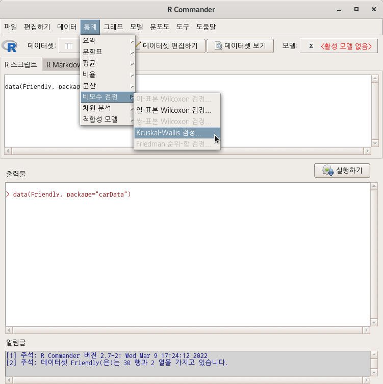
data(Friendly, package="carData")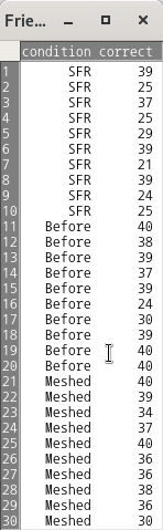
help("Friendly")| Friendly {carData} | R Documentation |
Format Effects on Recall
Description
The Friendly data frame has 30 rows and 2 columns. The data are from an experiment on subjects' ability to remember words based on the presentation format.
Usage
Friendly
Format
This data frame contains the following columns:
condition
A factor with levels: Before, Recalled words presented before others; Meshed, Recalled words meshed with others; SFR, Standard free recall.
correct
Number of words correctly recalled, out of 40 on final trial of the experiment.
Source
Friendly, M. and Franklin, P. (1980) Interactive presentation in multitrial free recall. Memory and Cognition 8 265–270 [Personal communication from M. Friendly].
References
Fox, J. (2016) Applied Regression Analysis and Generalized Linear Models, Third Edition. Sage.
Fox, J. and Weisberg, S. (2019) An R Companion to Applied Regression, Third Edition, Sage.