데이터 > 활성 데이터셋 > 활성 데이터셋의 합계 변수...
Data > Active data set > Aggregate variables in active data set...

데이터셋의 변수에는 수치형과 범주형, 문자형 등이 있다. 범주형 변수, 보통 R에서 factor(요인)형이라 부르는 변수를 기준으로 수치형 값들을 묶을 수 있다. 이 기능을 이해하기 위해서는 사용자가 수치형/요인형/문자형 등의 데이터유형에 대하여 알고 있어야 한다.
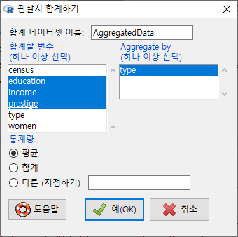
대화창에서 <Aggregate by (하나 이상 선택) > 에 등장하는 변수는 요인형 변수이며, 이 변수의 개별 요인형 사례를 기준으로 나머지 변수들의 정보가 묶이게 된다. 아래 화면의 type 변수는 요인형 변수이며, 나머지 변수는 수치형 변수인 것이다. <평균/합/다른 (지정하기)>의 옵션에서 선택할 수 있다. <합계 데이터셋 이름>은 'AggregateData'로 지정되어 있으나, 사용자가 임의로 바꿔서 사용할 수 있다.

예(OK)를 누르면, AggregatedData라는 데이터셋이 생성된다. <데이터셋 보기> 를 통해서 내부를 살펴보면, 직업 유형 (type)별로 직업의 권위에 대한 인식(prestige)의 평균 값이 보인다.

하나 이상의 수치형 변수를 선택해보자. Prestige 데이터셋에서 세개의 변수, education, income, prestige 를 선택하고 예(OK) 버튼을 누르자.
<데이터셋 보기> 버튼을 눌러 AggregatedData 내부를 살펴보면, 직업 유형 (type) 별로, 교육 연수(education), 연 수입(income), 권위 인식(prestige)의 평균 값이 확인할 수 있다.

아래 입력창은 두개의 합계 데이터셋을 만든다. AggregatedData, AggregatedData1인데, aggregate() 함수가 사용되는 것을 알 수 있다.

합계데이터셋 <- aggregate(수치형변수 ~ 요인형변수, data=활성데이터셋, FUN=mean)
?aggregate  #  stats 패키지의 aggregate 도움말 보기

## Compute the averages for the variables in 'state.x77', grouped
## according to the region (Northeast, South, North Central, West) that
## each state belongs to.
aggregate(state.x77, list(Region = state.region), mean)

## Compute the averages according to region and the occurrence of more
## than 130 days of frost.
aggregate(state.x77,
          list(Region = state.region,
               Cold = state.x77[,"Frost"] > 130),
          mean)
## (Note that no state in 'South' is THAT cold.)


## example with character variables and NAs
testDF <- data.frame(v1 = c(1,3,5,7,8,3,5,NA,4,5,7,9),
                     v2 = c(11,33,55,77,88,33,55,NA,44,55,77,99) )
by1 <- c("red", "blue", 1, 2, NA, "big", 1, 2, "red", 1, NA, 12)
by2 <- c("wet", "dry", 99, 95, NA, "damp", 95, 99, "red", 99, NA, NA)
aggregate(x = testDF, by = list(by1, by2), FUN = "mean")

# and if you want to treat NAs as a group
fby1 <- factor(by1, exclude = "")
fby2 <- factor(by2, exclude = "")
aggregate(x = testDF, by = list(fby1, fby2), FUN = "mean")


## Formulas, one ~ one, one ~ many, many ~ one, and many ~ many:
aggregate(weight ~ feed, data = chickwts, mean)
aggregate(breaks ~ wool + tension, data = warpbreaks, mean)
aggregate(cbind(Ozone, Temp) ~ Month, data = airquality, mean)
aggregate(cbind(ncases, ncontrols) ~ alcgp + tobgp, data = esoph, sum)

## Dot notation:
aggregate(. ~ Species, data = iris, mean)
aggregate(len ~ ., data = ToothGrowth, mean)

## Often followed by xtabs():
ag <- aggregate(len ~ ., data = ToothGrowth, mean)
xtabs(len ~ ., data = ag)


## Compute the average annual approval ratings for American presidents.
aggregate(presidents, nfrequency = 1, FUN = mean)
## Give the summer less weight.
aggregate(presidents, nfrequency = 1,
FUN = weighted.mean, w = c(1, 1, 0.5, 1))'Data > Active data set' 카테고리의 다른 글
| 11. Stack variables in active data set... (0) | 2019.09.08 |
|---|---|
| 10. Remove row(s) from active data set... (0) | 2019.09.08 |
| 8. Sort active data set... (6) | 2019.09.08 |
| 7. Subset active data set... (0) | 2019.09.08 |
| 6. Set case names... (0) | 2019.09.08 |