통계 > 차원 분석 > 군집 분석 > 위계 군집화를 데이터셋에 추가하기...

Statistics > Dimensional Analysis > Cluster Analysis > Add hierarchical clustering to data set...
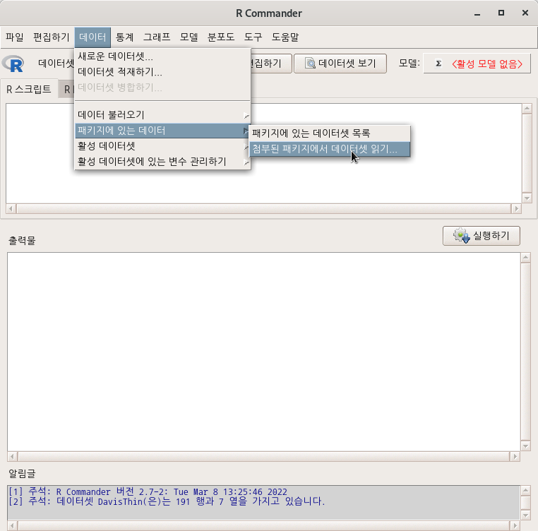
Linux 사례 (MX 21)

 ' 통계 > 차원 분석 > 군집 분석 > 위계 군집 분석...' 기능을 진행했다고 하자. 그 다음에 <위계군집화를 데이터 셋에 추가하기...>를 이용할 수 있다. <군집의 수:>를 3으로 변경하자. 그리고 예(OK) 버튼을 누르면, hclus.label라는 변수가 USArrests 데이터셋에 추가된다.

Linux 사례 (MX 21)

R Commander 상단에 있는 <데이터셋 보기> 버튼을 눌러보자. 아래와 같이 데이터셋의 내부 구성이 보일 것이다. hclus.label 변수가 추가되어 있음을 확인할 수 있다:

Linux 사례 (MX 21)

통계 > 차원 분석 > 군집 분석 > 위계 군집화 요약하기...

Statistics > Dimensional analysis > Cluster analysis > Summarizing hierarchical clustering...

Linux 사례 (MX 21)

'통계 > 차원 분석 > 군집 분석 > 위계 군집 분석'을 하였다고 하자. 그 다음에는 <위계 군집화 요약하기...> 기능을 사용할 수 있다.

https://rcmdr.kr/172


5.2. Hierarchical cluster analysis...

통계 > 차원 분석 > 군집 분석 > 위계 군집 분석... Statistics > Dimensional analysis > Cluster analysis > Hierarchical cluster analysis... datasets 패키지에 있는 USArrests 데이터셋을 활용해서, 위계..

rcmdr.kr

<위계적 군집 요약> 창에서 <군집의 수>를 3으로 변경해보자. <군집 요약 인쇄하기>, <군집 행렬도(Bi-plot)> 등이 선택되어 있는 것을 점검하자.

Linux 사례 (MX 21)

예(OK) 버튼을 누르면, 아래와 같은 그래픽 창이 등장한다.

Linux 사례 (MX 21)


summary(as.factor(cutree(HClust.1, k = 3))) # Cluster Sizes
by(model.matrix(~-1 + Assault + Murder + Rape + UrbanPop, USArrests), as.factor(cutree(HClust.1, k 
  = 3)), colMeans) # Cluster Centroids
biplot(princomp(model.matrix(~-1 + Assault + Murder + Rape + UrbanPop, USArrests)), xlabs = 
  as.character(cutree(HClust.1, k = 3)))

Linux 사례 (MX 21)

통계 > 차원 분석 > 군집 분석 > k-평균 군집 분석...

Statistics > Dimensional analysis > Cluster analysis > k-means cluster analysis...

Windows 사례 (10 Pro)

datasets 패키지에서 제공하는 USArrests 데이터셋을 이용해보자.

https://rcmdr.tistory.com/144


USArrests 데이터셋

datasets > USArrests data(USArrests, package="datasets") R Commander 화면 상단에서 <데이터셋 보기> 버튼을 누르면 아래와 같은 내부 구성을 확인할 수 있다. help("USArrests") USArrests {datasets} R Do..

rcmdr.kr

데이터셋에 포함된 네개의 변수를 모두 선택한다.

Windows 사례 (10 Pro)

<선택기능> 창에서, 군집의 수를 3개, 초기값의 수를 5번으로, 최대 반복 횟수를 5회로 정해보자. 데이터셋에 추가될 변수 이름이 KMeans가 될 것이다. 아래 있는 선택사항에서 데이터셋에 군집 할당하기를 선택한다.

Windows 사례 (10 Pro)

위 화면에서 선택된 군집 행렬도(Bi-plot)이 아래와 같이 생산된다.

Windows 사례 (10 Pro)

USArrests 데이터셋에 변수 KMeans가 추가될 것이다. R Commander 상단에 있는 <데이터셋 보기> 버튼을 눌러보자. KMeans 변수는 요인형으로 1, 2, 3 이라는 세개의 군집을 표시한다.

Windows 사례 (10 Pro)

아래 화면은 다소 복잡해보일 것이다. 그러나 객체 .cluster가 만들어졌으며, 그 객체안에 있는 $size, $withinss, $tot.withinss, $betweenss 등의 정보를 차례를 보여준다고 생각하자.  그리고 biplot을 생산하고, USArrests 데이터셋에 KMeans라는 변수를 추가하는 것이다.

'Statistics > Dimensional analysis' 카테고리의 다른 글

5.3. Summarize hierarchical clustering...  (0) 2022.03.20
5.2. Hierarchical cluster analysis...  (0) 2022.03.20
3. factor analysis...  (0) 2022.03.08
2. Principal-components analysis...  (0) 2022.03.08
1. Scale reliability...  (0) 2022.03.08

통계 > 차원 분석 > 주-성분 분석...

Statistics > Dimensional analysis > Principal-components analysis...

Linux 사례 (MX 21)

<주성분 분석> 메뉴 창에서 <변수 (두개 이상 선택)> 에서 4개의 변수를 모두 선택해보자.

Linux 사례 (MX 21)

<선택기능> 창에서 기본 설정되어 있는 기능을 기억하자.

Linux 사례 (MX 21)

local({
  .PC <- princomp(~Assault+Murder+Rape+UrbanPop, cor=TRUE, data=USArrests)
  cat("\nComponent loadings:\n")
  print(unclass(loadings(.PC)))
  cat("\nComponent variances:\n")
  print(.PC$sd^2)
  cat("\n")
  print(summary(.PC))
})


Linux 사례 (MX 21)


.PC <- princomp(~Assault+Murder+Rape+UrbanPop, cor=TRUE, data=USArrests)
plot(.PC)

Linux 사례 (MX 21)

biplot(.PC)

Linux 사례(MX 21)

'Statistics > Dimensional analysis' 카테고리의 다른 글

5.3. Summarize hierarchical clustering...  (0) 2022.03.20
5.2. Hierarchical cluster analysis...  (0) 2022.03.20
5.1. k-means cluster analysis...  (0) 2022.03.18
3. factor analysis...  (0) 2022.03.08
1. Scale reliability...  (0) 2022.03.08

datasets::USArrests()

Linux 사례(MX 21)
Linux 사례 (MX 21)

data(USArrests, package="datasets")

R Commander 화면 상단에서 <데이터셋 보기> 버튼을 누르면 아래와 같은 내부 구성을 확인할 수 있다.

Linux 사례 (MX 21)

help("USArrests")

USArrests {datasets} R Documentation

Violent Crime Rates by US State

Description

This data set contains statistics, in arrests per 100,000 residents for assault, murder, and rape in each of the 50 US states in 1973. Also given is the percent of the population living in urban areas.

Usage

USArrests

Format

A data frame with 50 observations on 4 variables.

[,1] Murder numeric Murder arrests (per 100,000)
[,2] Assault numeric Assault arrests (per 100,000)
[,3] UrbanPop numeric Percent urban population
[,4] Rape numeric Rape arrests (per 100,000)

Note

USArrests contains the data as in McNeil's monograph. For the UrbanPop percentages, a review of the table (No. 21) in the Statistical Abstracts 1975 reveals a transcription error for Maryland (and that McNeil used the same “round to even” rule that R's round() uses), as found by Daniel S Coven (Arizona).

See the example below on how to correct the error and improve accuracy for the ‘<n>.5’ percentages.

Source

World Almanac and Book of facts 1975. (Crime rates).

Statistical Abstracts of the United States 1975, p.20, (Urban rates), possibly available as https://books.google.ch/books?id=zl9qAAAAMAAJ&pg=PA20.

References

McNeil, D. R. (1977) Interactive Data Analysis. New York: Wiley.

See Also

The state data sets.

Examples

summary(USArrests)

require(graphics)
pairs(USArrests, panel = panel.smooth, main = "USArrests data")

## Difference between 'USArrests' and its correction
USArrests["Maryland", "UrbanPop"] # 67 -- the transcription error
UA.C <- USArrests
UA.C["Maryland", "UrbanPop"] <- 76.6

## also +/- 0.5 to restore the original  <n>.5  percentages
s5u <- c("Colorado", "Florida", "Mississippi", "Wyoming")
s5d <- c("Nebraska", "Pennsylvania")
UA.C[s5u, "UrbanPop"] <- UA.C[s5u, "UrbanPop"] + 0.5
UA.C[s5d, "UrbanPop"] <- UA.C[s5d, "UrbanPop"] - 0.5

## ==> UA.C  is now a *C*orrected version of  USArrests

[Package datasets version 4.1.0 Index]

'Dataset_info > USArrests' 카테고리의 다른 글

USArrests 데이터셋 예제  (0) 2022.06.25

+ Recent posts