?swiss # swiss 데이터셋 도움말 보기
# 아래는 example(swiss) 입니다.
require(stats); require(graphics)
pairs(swiss, panel = panel.smooth, main = "swiss data",
col = 3 + (swiss$Catholic > 50))
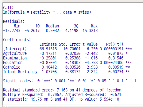
summary(lm(Fertility ~ . , data = swiss))
linux 사례 (MX 21)
pairs(swiss, panel = panel.smooth, main = "swiss data",
      col = 3 + (swiss$Catholic > 50))

pairs(swiss, panel = panel.smooth, main = "swiss data")  # 두 그래프를 비교해 보기
Linux 사례 (MX 21)Linux 사례 (MX 21)
LinearModel.1 <- lm(Fertility ~ . , data = swiss)
summary(LinearModel.1)
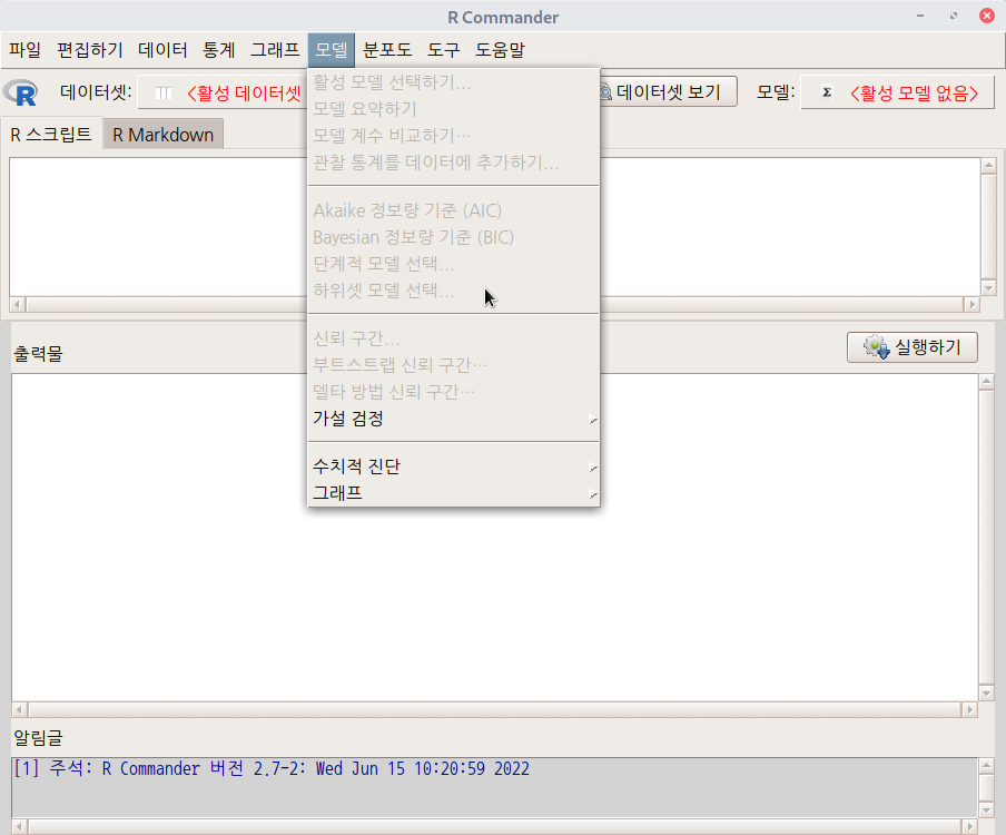
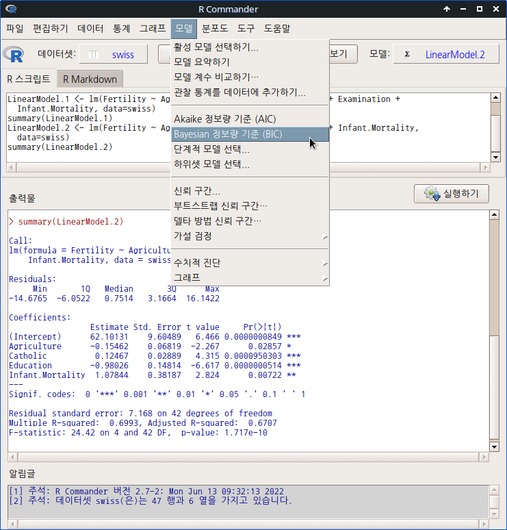
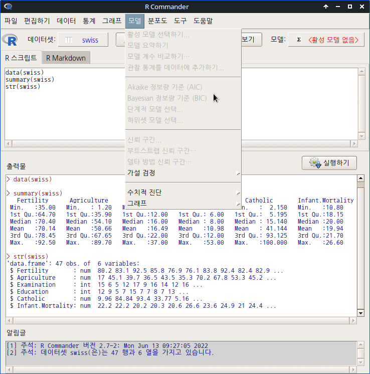
모델 > 하위셋 모델 선택... Models > Subset model selection...
Linux 사례 (MX 21)
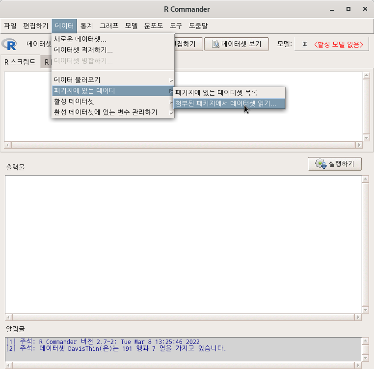
datasets 패키지에 있는 swiss 데이터셋으로 연습해보자. swiss 데이터셋을 불러온다. '데이터 > 패키지에 있는 데이터 > 첨부된 패키지에서 데이터셋 읽기' 메뉴 기능을 선택하여 datasets 패키지에 있는 swiss 데이터셋을 찾고 선택한다. https://rcmdr.tistory.com/184
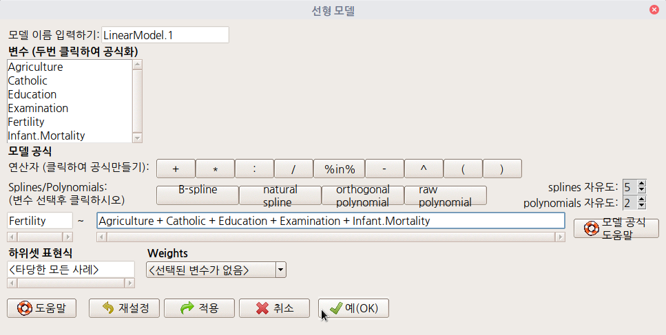
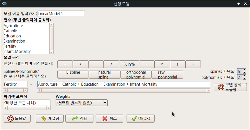
'통계 > 적합성 모델 > 선형 모델...' 메뉴 기능을 사용하여 swiss 데이터셋의 변수들 중에서 Fertility를 반응변수로, 나머지를 추천된 설명변수 후보로 가정하고, 선형 모델을 아래와 같이 만든다.
Linux 사례 (MX 21)
data(swiss, package="datasets") # swisss 데이터셋 불러오기
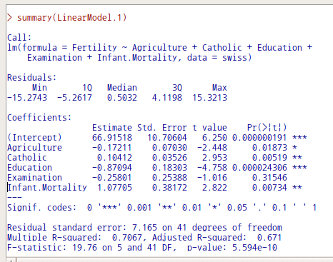
LinearModel.1 <- lm(Fertility ~ Agriculture + Catholic + Education + Examination +
Infant.Mortality, data=swiss) # 문제의식과 연관된 설명변수 후보들을 모두 선택하여 모형만들기
summary(LinearModel.1)
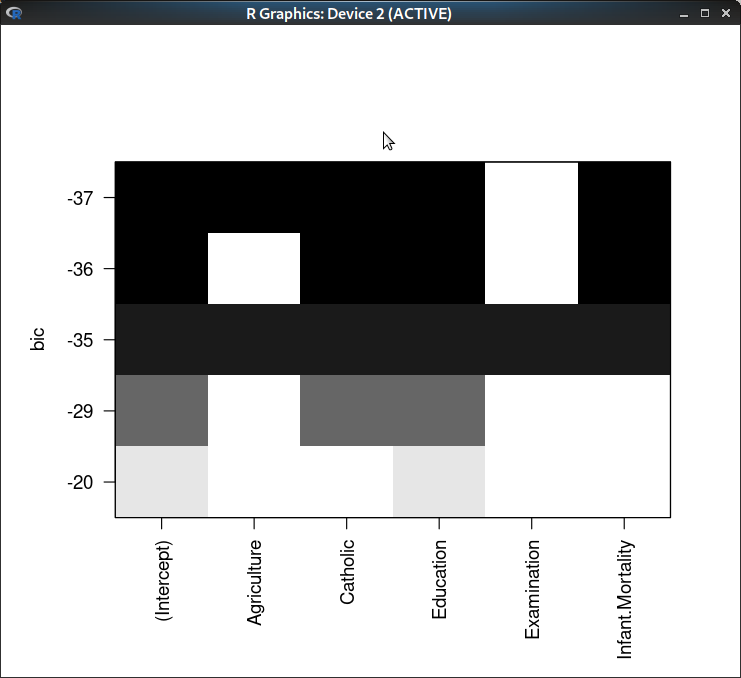
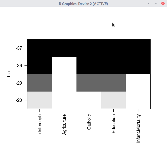
plot(regsubsets(Fertility ~ Agriculture + Catholic + Education + Examination +
Infant.Mortality, data=swiss, nbest=1, nvmax=6), scale='bic')
# 하위셋 모델 선택 그림 만들기
Linux 사례 (MX 21)
그래프에서 bic값이 가장 작은 숫자를 찾고, 이것과 연결된 설명변수 후보들 목록을 살펴보자. 검은색으로 표현된 것은 포함된 것, 흰색(공백)으로 표현된 것은 비포함된 것, 다른 말로 제거되어야 할 것이다. 그래프에서는 Examination 변수가 포함되지 않은 모형의 bic 값이 가장 작은 것을 알려준다.
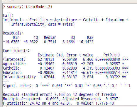
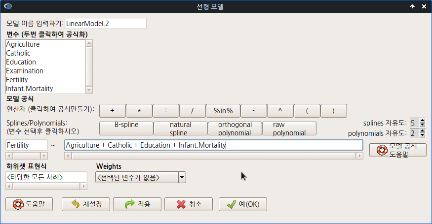
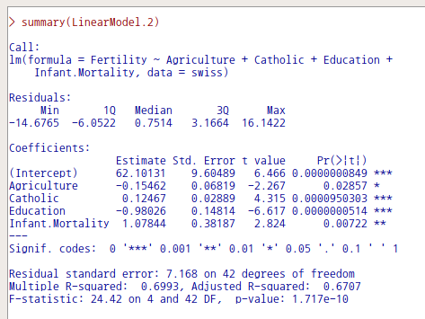
LinearModel.2 <- lm(Fertility ~ Agriculture + Catholic + Education + Infant.Mortality,
  data=swiss)              # Examination 변수를 제외한 추천 모형 만들기
summary(LinearModel.2)     # LinearModel.2의 요약 정보 보기
plot(regsubsets(Fertility ~ Agriculture + Catholic + Education + Infant.Mortality,
  data=swiss, nbest=1, nvmax=5), scale='bic')
                           # 추천된 하위셋 모델 점검하는 그림 만들기
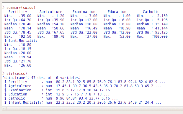
datasets 패키지에 있는 swiss 데이터셋은 1880년대 스위스 지방의 출산율과 사회경제적인 요인들에 대한 정보를 담고있다. 출산율(Fertility)에 영향을 미치는 요인들을 찾고, 설명력 높은 모형을 선택하고자 하는 과정이 필요하다. 다중회귀분석 기법을 활용한 선형모델을 만들고 계산하였다고 가정하자.
LinearModel.1과 LinearModel.2를 비교해보면, 설명변수에 Examination이 포함되어 있는가 여부이다. Examination 변수는 스위스의 지방별로 'draftees receiving highest mark on army examination'의 %를 사례값으로 담고 있다. 두 모형의 분석결과, 특히 Examination 변수의 유무에 따른 차이를 꼼꼼히 살펴보자.
LinearModel.1을 살펴보면, Examination 변수는 Fertility 변수에 유의미한 영향력을 미친다고 보기 어렵다. 그렇다면, LinearModel.1과 LinearModel.2에서 어느 모형을 선택해야 하는가? 두 모형의 Multiple R-squared, Adjusted R-squared, F-statistic, p-value 등은 작은 차이를 나타낸다.
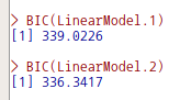
이 때 사용하는 방법의 하나가 Bayesian 정보량 기준 (BIC)이다. 'When comparing models fitted by maximum likelihood to the same data, the smaller the AIC or BIC, the better the fit.' 최대우도 또는 최대가능도 기법을 통하여 모형들을 비교할 때, 상대적으로 작은 값이 보다 적합도가 높다는 뜻이다. 결국 LinearModel.1과 LinearModel.2에서 어느 모형의 BIC 값이 더 작은가를 확인하여 보다 적합도가 높은 모형을 선택하고자 하는 것이다.
LinearModel.2의 BIC 값이 LinearModel.1의 BIC 값보다 미세하지만 더 작다. LinearModel.2가 더 적합도가 높은 모형이다라고 할 수 있다. 1880년대 스위스 지방의 출산율(Fertility)에 관한 사회경제적 요인들을 찾고, 설명변수들의 영향력을 점검할 때 Examination 변수를 제외한 모형을 사용하는 것이 바람직하다는 선택으로 이끌게 된다.
datasets 패키지에 있는 swiss 데이터셋은 1880년대 스위스 지방의 출산율과 사회경제적인 요인들에 대한 정보를 담고있다. 출산율(Fertility)에 영향을 미치는 요인들을 찾고, 설명력 높은 모형을 선택하고자 하는 과정이 필요하다. 다중회귀분석 기법을 활용한 선형모델을 만들고 계산하였다고 가정하자.
LinearModel.1과 LinearModel.2를 비교해보면, 설명변수에 Examination이 포함되어 있는가 여부이다. Examination 변수는 스위스의 지방별로 'draftees receiving highest mark on army examination'의 %를 사례값으로 담고 있다. 두 모형의 분석결과, 특히 Examination 변수의 유무에 따른 차이를 꼼꼼히 살펴보자.
LinearModel.1을 살펴보면, Examination 변수는 Fertility 변수에 유의미한 영향력을 미친다고 보기 어렵다. 그렇다면, LinearModel.1과 LinearModel.2에서 어느 모형을 선택해야 하는가? 두 모형의 Multiple R-squared, Adjusted R-squared, F-statistic, p-value 등은 작은 차이를 나타낸다.
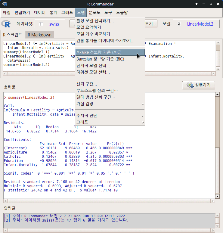
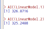
이 때 사용하는 방법의 하나가 Akaike 정보량 기준 (AIC)이다. 'When comparing models fitted by maximum likelihood to the same data, the smaller the AIC or BIC, the better the fit.' 최대우도 또는 최대가능도 기법을 통하여 모형들을 비교할 때, 상대적으로 작은 값이 보다 적합도가 높다는 뜻이다. 결국 LinearModel.1과 LinearModel.2에서 어느 모형의 AIC 값이 더 작은가를 확인하여 보다 적합도가 높은 모형을 선택하고자 하는 것이다.
LinearModel.2의 AIC 값이 LinearModel.1의 AIC 값보다 미세하지만 더 작다. LinearModel.2가 더 적합도가 높은 모형이다라고 할 수 있다. 1880년대 스위스 지방의 출산율(Fertility)에 관한 사회경제적 요인들을 찾고, 설명변수들의 영향력을 점검할 때 Examination 변수를 제외한 모형을 사용하는 것이 바람직하다는 선택으로 이끌게 된다.
Swiss Fertility and Socioeconomic Indicators (1888) Data
Description
Standardized fertility measure and socio-economic indicators for each of 47 French-speaking provinces of Switzerland at about 1888.
Usage
swiss
Format
A data frame with 47 observations on 6 variables, each of which is in percent, i.e., in [0, 100].
[,1]
Fertility
Ig, ‘common standardized fertility measure’
[,2]
Agriculture
% of males involved in agriculture as occupation
[,3]
Examination
% draftees receiving highest mark on army examination
[,4]
Education
% education beyond primary school for draftees.
[,5]
Catholic
% ‘catholic’ (as opposed to ‘protestant’).
[,6]
Infant.Mortality
live births who live less than 1 year.
All variables but ‘Fertility’ give proportions of the population.
Details
(paraphrasing Mosteller and Tukey):
Switzerland, in 1888, was entering a period known as the demographic transition; i.e., its fertility was beginning to fall from the high level typical of underdeveloped countries.
The data collected are for 47 French-speaking “provinces” at about 1888.
Here, all variables are scaled to [0, 100], where in the original, all but "Catholic" were scaled to [0, 1].
They state that variables Examination and Education are averages for 1887, 1888 and 1889.
Source
Project “16P5”, pages 549–551 in
Mosteller, F. and Tukey, J. W. (1977) Data Analysis and Regression: A Second Course in Statistics. Addison-Wesley, Reading Mass.
indicating their source as “Data used by permission of Franice van de Walle. Office of Population Research, Princeton University, 1976. Unpublished data assembled under NICHD contract number No 1-HD-O-2077.”
References
Becker, R. A., Chambers, J. M. and Wilks, A. R. (1988) The New S Language. Wadsworth & Brooks/Cole.
Examples
require(stats); require(graphics)
pairs(swiss, panel = panel.smooth, main = "swiss data",
      col = 3 + (swiss$Catholic > 50))
summary(lm(Fertility ~ . , data = swiss))