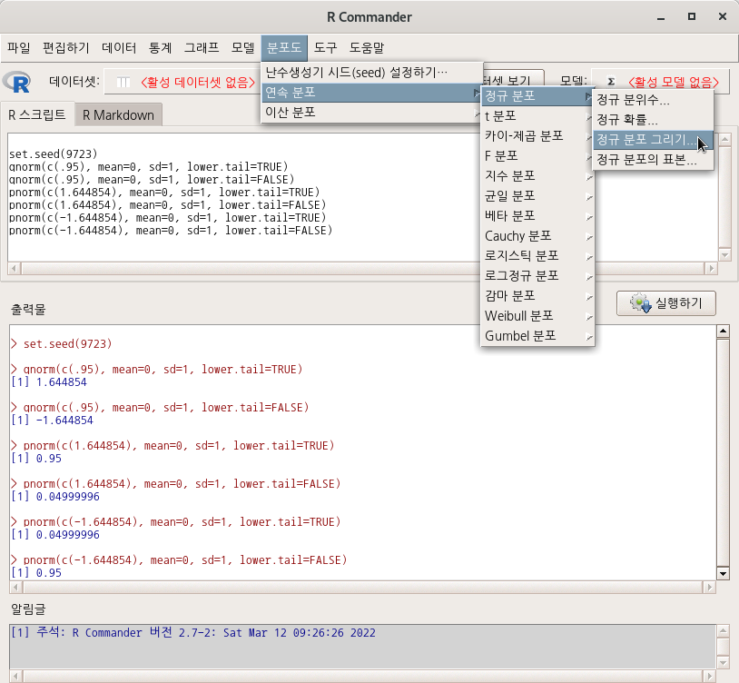
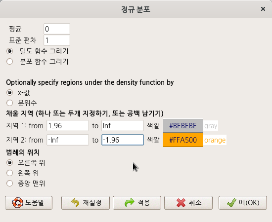
분포도 > 연속 분포 > 정규 분포 > 정규 분포 그리기...
Distributions > Continuous distributions > Normal distribution > Plot normal distribution...
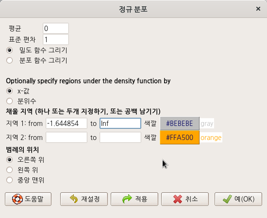
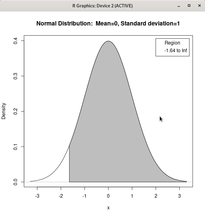
<밀도 함수 그리기 (Plot density function)>를 선택하고 <x-값>을 선택한 상황에서 몇 몇 사례를 만들어본다.
local({
  .x <- seq(-3.291, 3.291, length.out=1000)
  plotDistr(.x, dnorm(.x, mean=0, sd=1), cdf=FALSE, xlab="x", ylab="Density",
  main=paste("Normal Distribution:  Mean=0, Standard deviation=1"), regions=list(c(-1.644854, Inf)),
  col=c('#BEBEBE', '#FFA500'), legend.pos='topright')
})

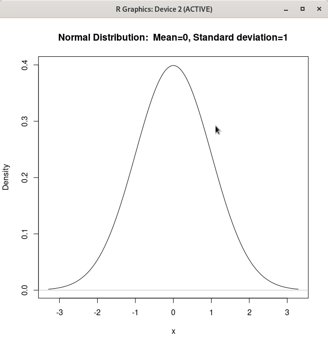
local({
  .x <- seq(-3.291, 3.291, length.out=1000)
  plotDistr(.x, dnorm(.x, mean=0, sd=1), cdf=FALSE, xlab="x", ylab="Density",
  main=paste("Normal Distribution:  Mean=0, Standard deviation=1"))
})
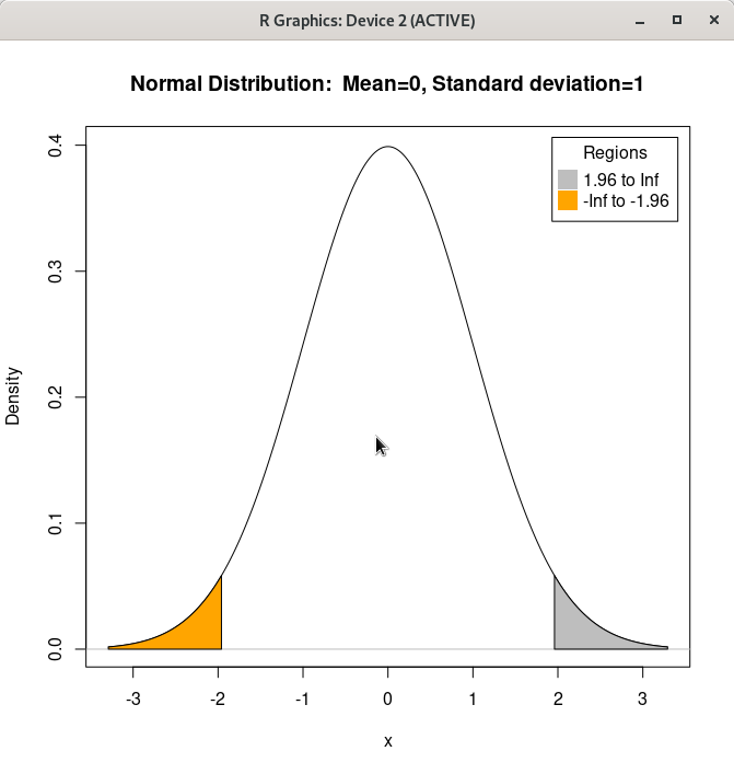
local({
  .x <- seq(-3.291, 3.291, length.out=1000)
  plotDistr(.x, dnorm(.x, mean=0, sd=1), cdf=FALSE, xlab="x", ylab="Density",
  main=paste("Normal Distribution:  Mean=0, Standard deviation=1"), regions=list(c(1.96, Inf), c(-Inf,
  -1.96)), col=c('#BEBEBE', '#FFA500'), legend.pos='topright')
})
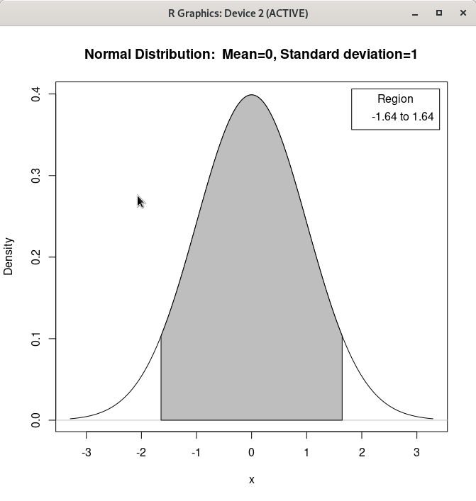
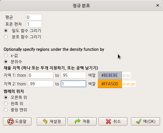
<밀도 함수 그리기 (Plot density function)>를 선택하고 <분위수>를 선택한 상황에서 몇 몇 사례를 만들어본다.

<분위수>에 입력할 수 있는 범위는 0에서 1까지의 확률이다. 이 범위 안에 들어오는 숫자는 아래 명령문 내부 regions에서 보이듯이 분위수로 전환된다.
local({
  .x <- seq(-3.291, 3.291, length.out=1000)
  plotDistr(.x, dnorm(.x, mean=0, sd=1), cdf=FALSE, xlab="x", ylab="Density",
  main=paste("Normal Distribution:  Mean=0, Standard deviation=1"), regions=list(c(-1.64485362695147,
  1.64485362695147)), col=c('#BEBEBE', '#FFA500'), legend.pos='topright')
})

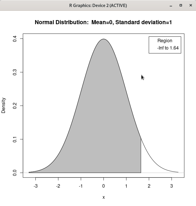
local({
  .x <- seq(-3.291, 3.291, length.out=1000)
  plotDistr(.x, dnorm(.x, mean=0, sd=1), cdf=FALSE, xlab="x", ylab="Density",
  main=paste("Normal Distribution:  Mean=0, Standard deviation=1"), regions=list(c(-Inf,
  1.64485362695147)), col=c('#BEBEBE', '#FFA500'), legend.pos='topright')
})
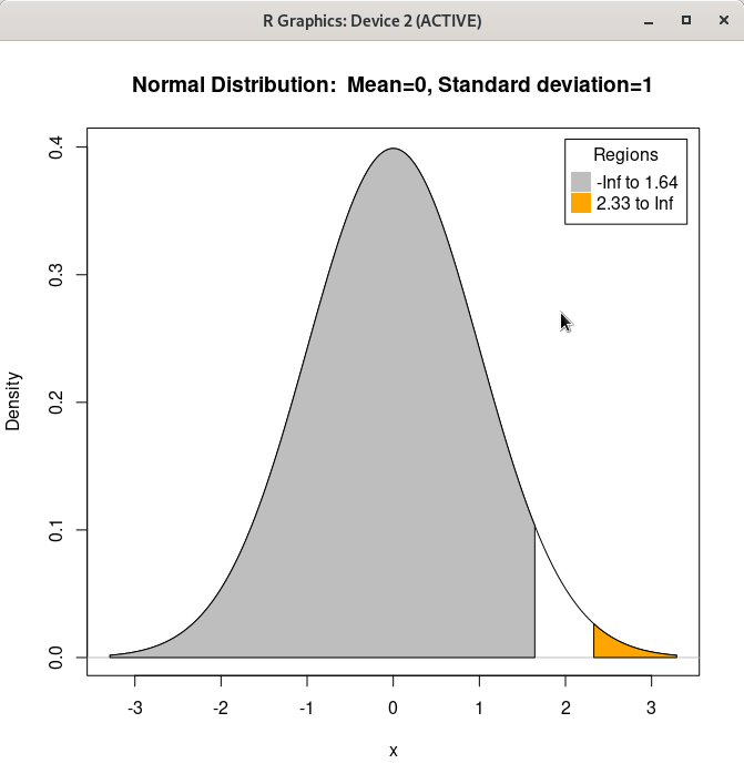
local({
  .x <- seq(-3.291, 3.291, length.out=1000)
  plotDistr(.x, dnorm(.x, mean=0, sd=1), cdf=FALSE, xlab="x", ylab="Density",
  main=paste("Normal Distribution:  Mean=0, Standard deviation=1"), regions=list(c(-Inf,
  1.64485362695147), c(2.32634787404084, Inf)), col=c('#BEBEBE', '#FFA500'), legend.pos='topright')
})
'Distributions > Continuous distributions' 카테고리의 다른 글
| 1.4. Sample from normal distribution... (0) | 2022.03.12 |
|---|---|
| 1.2. Normal probabilities... (0) | 2022.03.12 |
| 1.1. Normal quantiles... (0) | 2022.03.12 |